19 Day 17: Zones
19.1 Technologies/Techniques
- More
{sf}wrangling - Region shapefiles & piracy data from the
{asam}package {ggplot2}/geom_sf()
19.2 Data Source: NIMA/NGA Zones & ASAM PIRATE! Data
I pondered a bit on what to do for today’s challenge since there are many types of zones: environmental… temperate… time…
After checking out some of my older blog posts, I went back over to my {asam} package (we used this in a previous challenge) which has a shapefile I made from the National Imagery and Mapping Agency (NIMA)56/National Geospatial-Intelligence Agency (NGA) Catalog of Hydrographic Products.
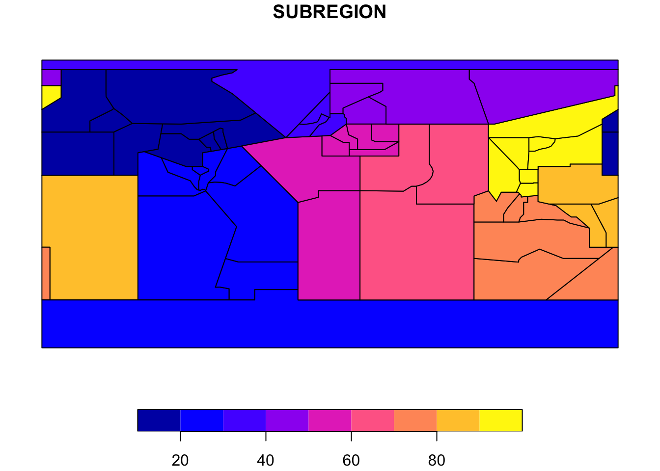
There are 9 ASAM global regions and 52 ASAM global subregions. These are referenced in REGION and SUBREGION fields in the returned {sf} object. I’m classifying these as zones for the sake of this challenge.
What is an NIMA/ASAM region/subregion? Well, for their use, the world is divided into nine regions: each corresponding to the geographic limits of one of the nine regions in the NIMA catalog. Each region is further divided into numbered subregions. The first digit of all five-digit chart numbers indicates the geographic region while the first two digits of all five-digit chart numbers refer to the geographic subregion. That may be super dry commentary, but at least they’ve got a data strategy.
library(sf)
library(asam)
library(albersusa)
library(rnaturalearth)
library(hrbrthemes)
library(tidyverse)
We’ll grab the NIMA/NGA zones:
and, take a look at the subregions:
Now, we’ll read in pirate data again and turn it into a points geometry object:
if (!file.exists(here::here("data/incidents-17.rds"))) {
  incidents <- read_asam()
  incidents <- st_as_sf(incidents, coords = c("longitude", "latitude"), crs = us_longlat_proj)
  saveRDS(incidents, here::here("data/incidents-17.rds"))
}

incidents <- readRDS(here::here("data/incidents-17.rds"))

glimpse(incidents)
## Observations: 7,843
## Variables: 8
## $ reference   <chr> "2019-73", "2019-72", "2019-75", "2019-74", "2019-76", "2…
## $ date        <date> 2019-09-30, 2019-09-28, 2019-09-23, 2019-09-23, 2019-09-…
## $ navArea     <chr> "XI", "XI", "II", "XI", "II", "XI", "II", "XI", "IV", "II…
## $ subreg      <chr> "71", "92", "57", "72", "51", "71", "51", "71", "26", "57…
## $ hostility   <chr> "Five Armed robbers", "Two High-speed boats", NA, "Seven …
## $ victim      <chr> "Bulk Carrier", "Bulk Carrier", NA, "two fishing vessels"…
## $ description <chr> ", SINGAPORE STRAITS. DECK CREW ON ROUTINE ROUNDS ONBOARD…
## $ geometry    <POINT [°]> POINT (103.65 1.045), POINT (119.7283 5.325), POINT…
Keen eyes will see a subreg field in that tidy {sf} object, so we could just count() by that, but we’lre going to do some work and use st_intersection() to identify the subregion by point.
zones %>%
  left_join(
    st_intersection(incidents, select(zones, SUBREGION)) %>%
      as_tibble() %>%
      count(SUBREGION)
  ) -> locs

glimpse(locs)
## Observations: 58
## Variables: 8
## $ OBJECTID   <int> 1, 2, 3, 4, 5, 6, 7, 8, 9, 10, 11, 12, 13, 14, 15, 16, 17,…
## $ ID         <int> 1, 2, 3, 4, 5, 6, 7, 8, 9, 10, 11, 12, 13, 14, 15, 16, 17,…
## $ SUBREGION  <int> 83, 19, 17, 18, 21, 28, 27, 11, 26, 25, 12, 13, 14, 15, 16…
## $ REGION     <int> 8, 1, 1, 1, 2, 2, 2, 1, 2, 2, 1, 1, 1, 1, 1, 9, 4, 7, 2, 2…
## $ Shape_Leng <dbl> 275.90637, 144.08198, 66.67966, 116.55910, 123.27130, 70.8…
## $ Shape_Area <dbl> 4513.12768, 1216.84278, 248.73010, 692.64299, 672.56328, 1…
## $ n          <int> 9, NA, NA, 1, 13, 38, 7, 1, 82, 122, 1, 1, NA, NA, NA, 1, …
## $ geometry   <POLYGON [°]> POLYGON ((-180 -26.98819, -..., POLYGON ((-180 17.…

# or:

left_join(
  mutate(zones, SUBREGION = as.character(SUBREGION)),
  count(incidents, subreg) %>%
    as_tibble() %>%
    select(SUBREGION = subreg, n)
) %>%
  glimpse()
## Observations: 58
## Variables: 8
## $ OBJECTID   <int> 1, 2, 3, 4, 5, 6, 7, 8, 9, 10, 11, 12, 13, 14, 15, 16, 17,…
## $ ID         <int> 1, 2, 3, 4, 5, 6, 7, 8, 9, 10, 11, 12, 13, 14, 15, 16, 17,…
## $ SUBREGION  <chr> "83", "19", "17", "18", "21", "28", "27", "11", "26", "25"…
## $ REGION     <int> 8, 1, 1, 1, 2, 2, 2, 1, 2, 2, 1, 1, 1, 1, 1, 9, 4, 7, 2, 2…
## $ Shape_Leng <dbl> 275.90637, 144.08198, 66.67966, 116.55910, 123.27130, 70.8…
## $ Shape_Area <dbl> 4513.12768, 1216.84278, 248.73010, 692.64299, 672.56328, 1…
## $ n          <int> 9, NA, NA, 1, 13, 38, 7, 1, 82, 122, 1, 1, NA, NA, NA, 1, …
## $ geometry   <POLYGON [°]> POLYGON ((-180 -26.98819, -..., POLYGON ((-180 17.…
We’ll also want to plot a normal world map so there’s some idea of where things are, so we’ll grab that from {rnaturalearth} as we’ve done quite a bit:
19.3 Drawing the Map
This is just like a choropleth map, but we’re filling zones vs states/countries. To mix things up a bit we’ll also put the counts in the zones at the zone centroid.
ggplot() +
  geom_sf(
    data = world, color = "#2b2b2b", size = 0.125, fill="#d9d9d9"
  ) +
  geom_sf(
    data = select(locs, SUBREGION, n), aes(fill = n),
    size = 0.125, alpha=1/2, color = "#b3000077"
  )  +
  geom_sf_text(
    data = select(locs, SUBREGION, n),
    aes(
      label = I(ifelse(is.na(n), "", scales::comma(n))),
      color = I(ifelse(n > 900, "black", "white")) # change text color depending on the background
    ),
    family = font_es_bold, size = 3.33 # putting a slightly bigger version below with the inverse color
  ) +
  geom_sf_text(
    data = select(locs, SUBREGION, n),
    aes(
      label = I(ifelse(is.na(n), "", scales::comma(n))),
      color = I(ifelse(n > 900, "white", "black")) # change text color depending on the background
    ),
    family = font_es_bold, size = 3.25 # put a slighly smaller version on top with the actual color
  ) +
  scale_fill_viridis_c(
    name = "Number of Anti-Shipping Incidents\n",
    option = "magma", direction = -1, na.value = "white",
    label = scales::comma
  ) +
  labs(
    x = NULL, y = NULL,
    title = "Total Anti-Shipping Activity since 1978 by Sub-Region Zone",
    subtitle = "Zones depicted with red border; counts are total incidents (mostly piracy)",
    caption = "Data source: {asam} • #30DayMapChallenge"
  ) +
  theme_ipsum_es(grid="") +
  theme(legend.position = "top") +
  theme(legend.key.width = unit(3, "lines")) +
  theme(legend.direction = "horizontal")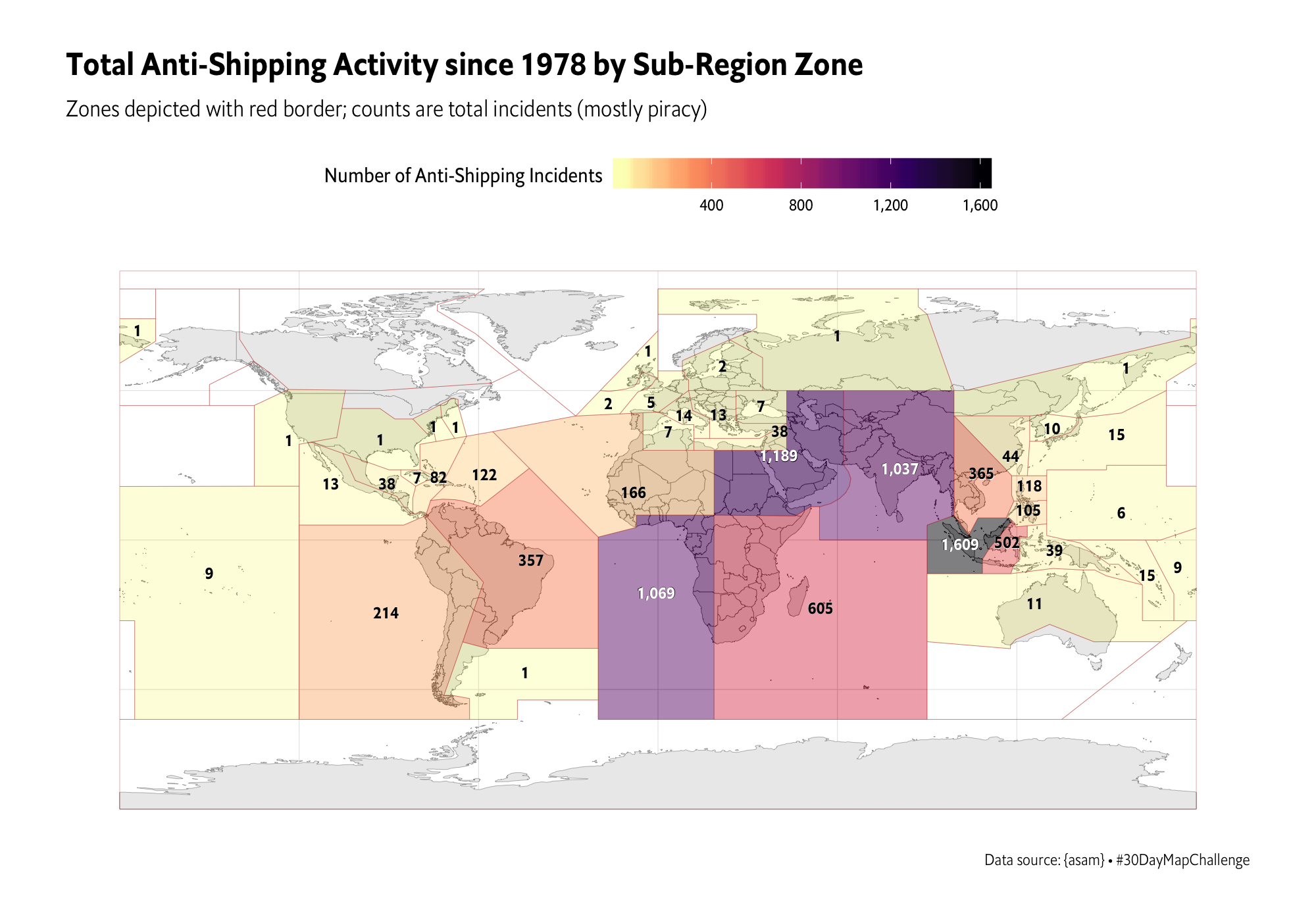
19.4 In Review
We layered a different shapefile on top of our standard world base shapefile and filled that with values based on computed point-in-polygon frequency.
19.5 Try This At Home
The {mapdeck} package lets you add custom layers like the zones shapefile. Use it to visualize the incidents.
Animate the map over time with a bar chart below it counting incidents by year.