11 Day 9: Yellow

11.1 Technologies/Techniques

R Simple Features {sf}
Generating your own data to put on a map
Using {rnaturalearth} basemaps
Using {ggplot2} geom_sf() to draw a basemap, geom_path() to draw lines and geom_ribbon() to make filled polygons
Making animations with {magick}

11.2 Data Source: Solar Terminator

The line on the surface of our planet that separates day and night is called the “terminator” and for today’s challenge I decided to create an animation of this line as it moves across the Earth. To do this, we need to compute the terminator for each hour.

Joe Gallagher⁴³ made an initial R script⁴⁴ to compute the terminator. I riffed off of this and made an Rcpp-based {terminator} package⁴⁵ that dramatically speeds up the calculations and makes the function easier to use since it’s in a package.

library(sf)
library(magick)
library(terminator)
library(rnaturalearth)
library(hrbrthemes)
library(tidyverse)

To see what the terminator() function does before making the final map, we’ll compute one terminator line for midday (GMT) and place it on a map:

ne_countries(scale = "medium", returnclass = "sf") %>%
  filter(name != "Antarctica") -> world

ggplot() +
  geom_sf(data = world, size = 0.125) +
  geom_path(
    data = terminator(as.integer((as.POSIXct(Sys.Date()) + (60*60*12))), -180, 180, 0.1),
    aes(lon, lat), size = 2
  ) +
  coord_sf(crs="+proj=longlat") +
  labs(x = NULL, y = NULL) +
  theme_minimal()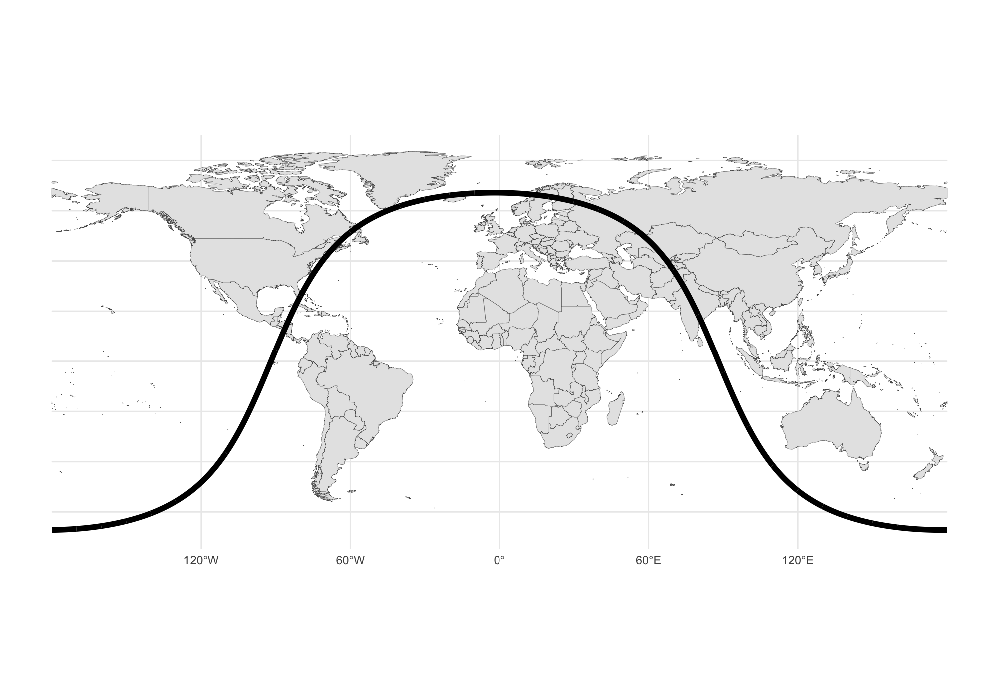

Note the use of geom_path() which forced us to re-project the world back to plain ol’ longlat in order to avoid messing with the unprojected longitude/latitude pairs from terminator()

11.3 Building Projected Terminators

We’ll use a different projection — cylindrical equal-earth⁴⁶ – this time just to mix things up a bit and also write a helper function to obtain pre-projected longitude/latitude points for our terminator lines:

# cylindrical equal-earth projection
proj <- "+proj=cea +lat_ts=37.5 +ellps=WGS84 +datum=WGS84 +units=m +no_defs +towgs84=0,0,0"

get_terms <- function(i) { # i is the hour of the day (GMT)

  terminator(as.integer((as.POSIXct(Sys.Date()) + (60*60*(i)))), -180, 180, 0.1) %>% # get a data frame of points
    st_as_sf(coords = c("lon", "lat"), crs = 4326, agr = "constant") %>% # make an {sf} object
    st_transform(crs = proj) %>% # project the points
    st_coordinates() %>% # get the coordinates back
    as_tibble() %>% # turn it back into a data frame
    set_names(c("lng", "lat"))

}

Rather than build complete polygons, we’ll cheat a bit and use geom_ribbon() to do that for us. The lat value of our line gives us the top (ymax) of the ribbon, so we just need to know the value for the bottom, which we can either look-up or compute:

st_as_sf(tibble(lon = 0, lat = -90), coords = c("lon", "lat"), crs = 4326, agr = "constant") %>%
  st_transform(crs = proj) %>%
  st_coordinates() %>%
  .[,2] -> bottom

bottom
## [1] -8011546

11.4 Drawing the Terminator Map (Part 1)

Let’s re-draw the GMT midday terminator map with a yellow ribbon:

  ggplot() +
    geom_sf(data = world, size = 0.125, fill = "#3B454A", color = "#b2b2b2") +
    geom_ribbon(
      data = get_terms(12), aes(lng, ymin = bottom, ymax = lat),
      fill = "#f9d71c", alpha = 1/6
    ) +
    coord_sf(crs = proj) +
    labs(
      x = NULL, y = NULL, title = sprintf("%02d:00", 12),
      caption = "Data source: {terminator} • #30DayMapChallenge"
    ) +
    theme_ft_rc(grid = "XY") +
    theme(plot.title = element_text(hjust = 0.5))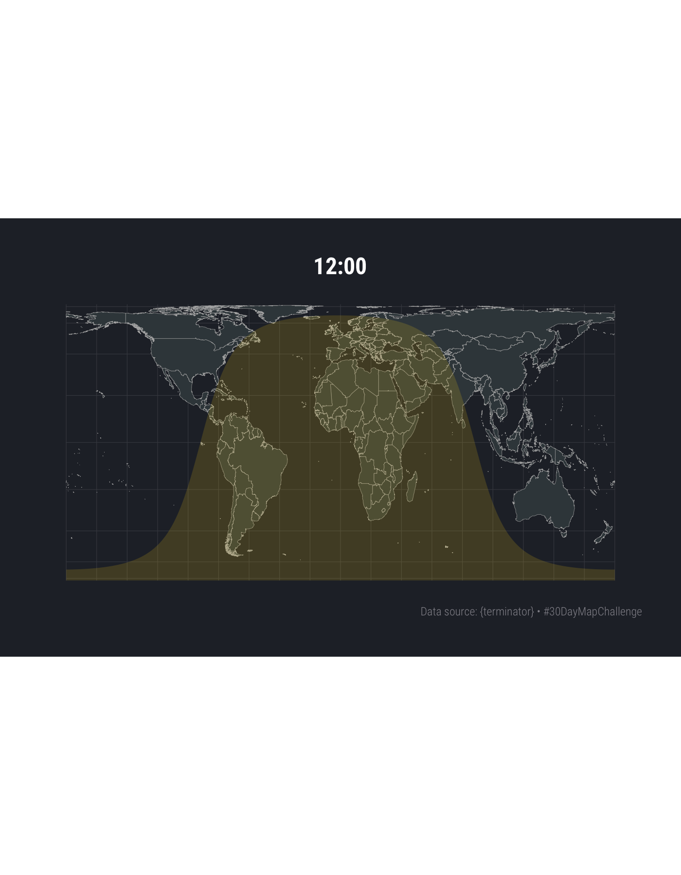

11.5 Drawing the Terminator Map (Part 2)

Now, we just follow the familiar-by-now {magick} animation idiom:"

img <- image_graph(width=1000*2, height=500*2, res=96)

pb <- progress_estimated(24)

for (i in 0:23) {

  pb$tick()$print()

  ggplot() +
    geom_sf(data = world, size = 0.125, fill = "#3B454A", color = "#b2b2b2") +
    geom_ribbon(
      data = get_terms(i), aes(lng, ymin = bottom, ymax = lat),
      fill = "#f9d71c", alpha = 1/6
    ) +
    coord_sf(crs = proj) +
    labs(
      x = NULL, y = NULL, title = sprintf("%02d:00", i),
      caption = "Data source: {terminator}\n<git.rud.is/hrbrmstr/y2019-30daymapchallenge> • #30DayMapChallenge"
    ) +
    theme_ft_rc(grid = "XY") +
    theme(plot.title = element_text(hjust = 0.5)) -> gg

  print(gg)

}

dev.off()

img <- image_animate(img)

image_write(img, here::here("img/terminus.gif"))

11.6 In Review

We mixed things up a bit and made our own data for this challenge along with trying out a new map projection. We also did some data frame to {sf} coordinate machinations in order to use our new projection.

11.7 Try This At Home

Flip the idiom (along with the basemap colors) and map night vs day.

Make {sf} polygons vs lines and plot the terminator on a {mapdeck} interactive map.