Data Source: Maine County Profiles
library(sf)
library(stringi)
library(hrbrthemes)
library(cartogram)
library(readxl)
library(tidyverse)
if (!file.exists(here::here("data/county-profiles.xlsx"))) {
download.file(
"https://www.maine.gov/labor/cwri/county-economic-profiles/Excel/CountyProfiles.xlsx",
here::here("data/county-profiles.xlsx")
)
}
st_read(here::here("data/me-counties.json"), stringsAsFactors=FALSE) %>%
st_set_crs(4326) %>%
st_transform(albersusa::us_laea_proj) -> me_counties
## Reading layer `cb_2015_maine_county_20m' from data source `/Users/hrbrmstr/books/30-day-map-challenge/data/me-counties.json' using driver `TopoJSON'
## Simple feature collection with 16 features and 10 fields
## geometry type: MULTIPOLYGON
## dimension: XY
## bbox: xmin: -71.08434 ymin: 43.05975 xmax: -66.9502 ymax: 47.45684
## epsg (SRID): NA
## proj4string: NA
read_excel(here::here("data/county-profiles.xlsx"), "Population") %>%
filter(Year == 2017, Geography == "County") %>%
janitor::clean_names() %>%
select(NAME = area_name, population) %>%
mutate(NAME = stri_replace_last_fixed(NAME, " Cty", "")) -> pop_raw
me_counties %>%
left_join(pop_raw, by = "NAME") -> me_pop
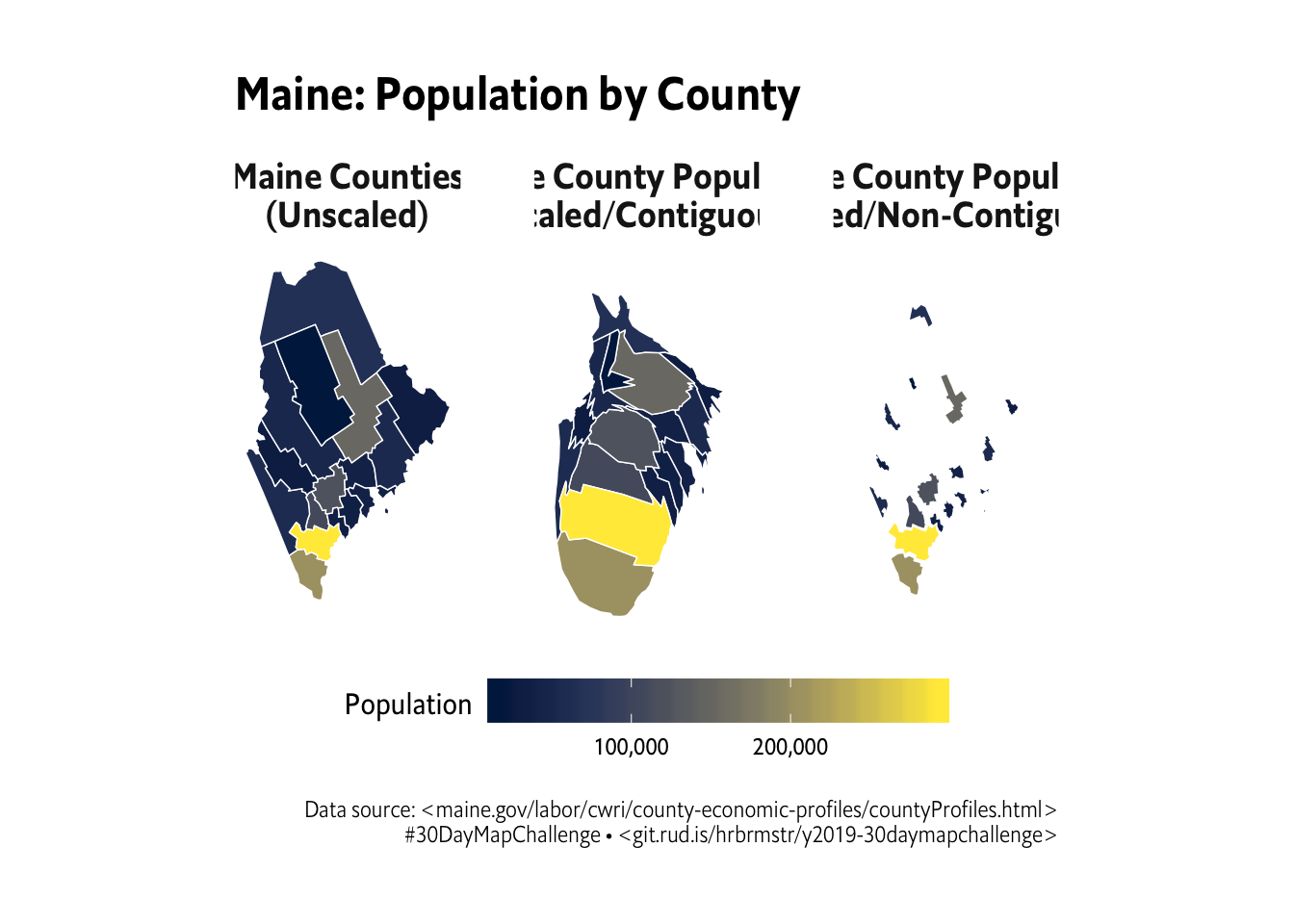
rbind(
me_pop %>%
mutate(title = "Maine Counties\n(Unscaled)") %>%
select(title, NAME, population, geometry),
cartogram_cont(me_pop, "population") %>%
mutate(title = "Maine County Population\n(Scaled/Contiguous)") %>%
select(title, NAME, population, geometry),
cartogram_ncont(me_pop, "population") %>%
mutate(title = "Maine County Population\n(Scaled/Non-Contiguous)") %>%
select(title, NAME, population, geometry)
) %>%
mutate(title = fct_inorder(title)) -> me_pop_scaled
ggplot() +
geom_sf(data = me_pop_scaled, aes(fill = population), color = "white", size = 0.25) +
facet_wrap(~title) +
scale_fill_viridis_c(
name = "Population\n", label=scales::comma, option = "cividis", direction = 1
) +
coord_sf(crs = albersusa::us_laea_proj, datum = NA) +
labs(
title = "Maine: Population by County",
caption = "Data source: <maine.gov/labor/cwri/county-economic-profiles/countyProfiles.html>\n#30DayMapChallenge • <git.rud.is/hrbrmstr/y2019-30daymapchallenge>"
) +
theme_ipsum_es(grid="", strip_text_family = font_es_bold, strip_text_size = 14) +
theme(strip.text = element_text(hjust = 0.5)) +
theme(legend.position = "bottom") +
theme(legend.key.width = unit(2.5, "lines"))
read_excel(here::here("data/county-profiles.xlsx"), "Industry Employment") %>%
janitor::clean_names() %>%
filter(
year == 2017,
period_type == "Annual",
level == 2,
ownership != "Total",
naics == 10
) %>%
select(NAME = area_name, ownership, total_wages, average_employment) %>%
mutate(NAME = stri_replace_last_fixed(NAME, " Cty", "")) %>%
left_join(pop_raw, "NAME") %>%
mutate(emp_pop = average_employment / population) -> emp
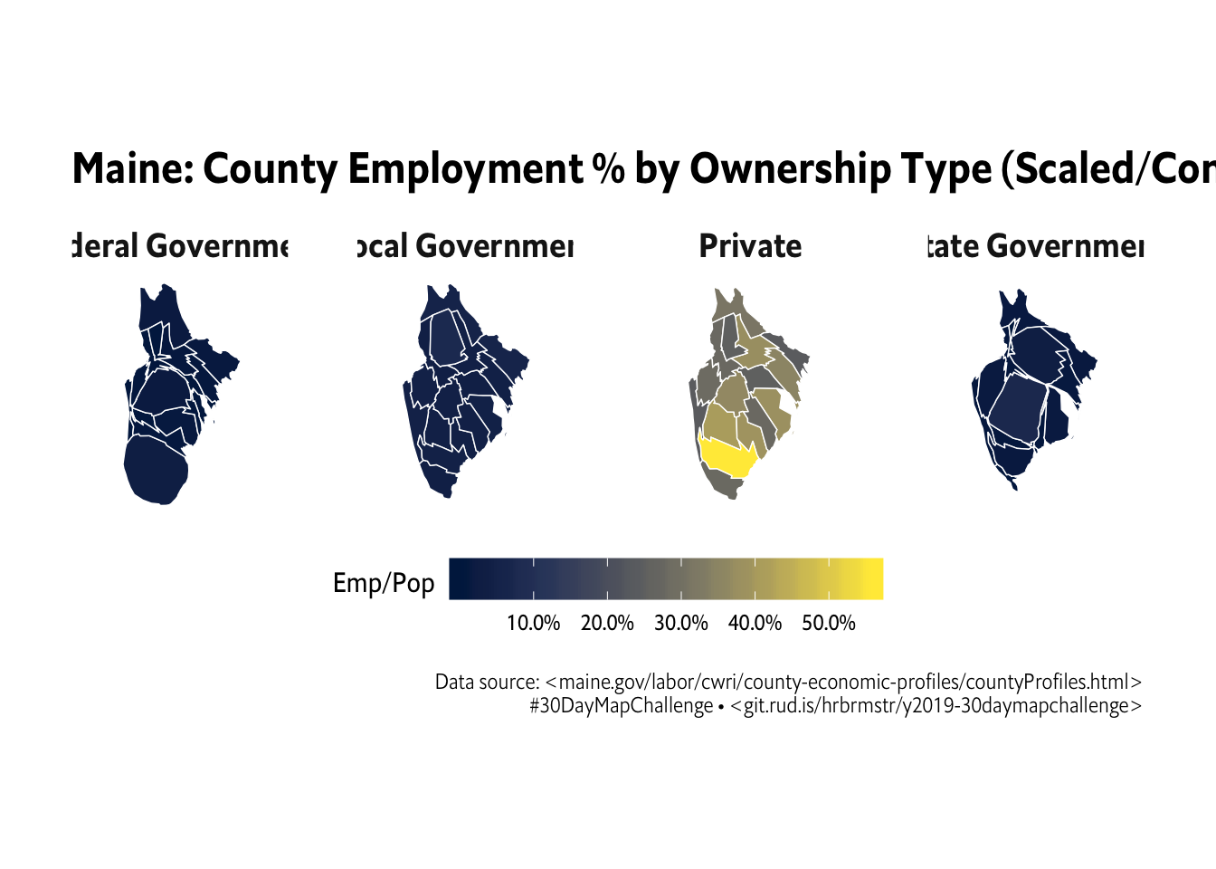
distinct(emp, ownership) %>%
pull(ownership) %>%
map(~{
left_join(me_counties, filter(emp, ownership == .x), "NAME") %>%
cartogram_cont("emp_pop")
}) %>%
do.call(rbind, .) %>%
ggplot() +
geom_sf(aes(fill = emp_pop), color = "white", size = 0.25) +
scale_x_continuous(expand = c(0, 100000)) +
scale_fill_viridis_c(
name = "Emp/Pop\n", label=scales::percent, option = "cividis", direction = 1
) +
coord_sf(crs = albersusa::us_laea_proj, datum=NA) +
facet_wrap(~ownership, ncol=4) +
labs(
title = "Maine: County Employment % by Ownership Type (Scaled/Contiguous)",
caption = "Data source: <maine.gov/labor/cwri/county-economic-profiles/countyProfiles.html>\n#30DayMapChallenge • <git.rud.is/hrbrmstr/y2019-30daymapchallenge>"
) +
theme_ipsum_es(grid="", strip_text_family = font_es_bold, strip_text_size = 14) +
theme(strip.text = element_text(hjust = 0.5)) +
theme(legend.position = "bottom") +
theme(legend.key.width = unit(2.5, "lines"))
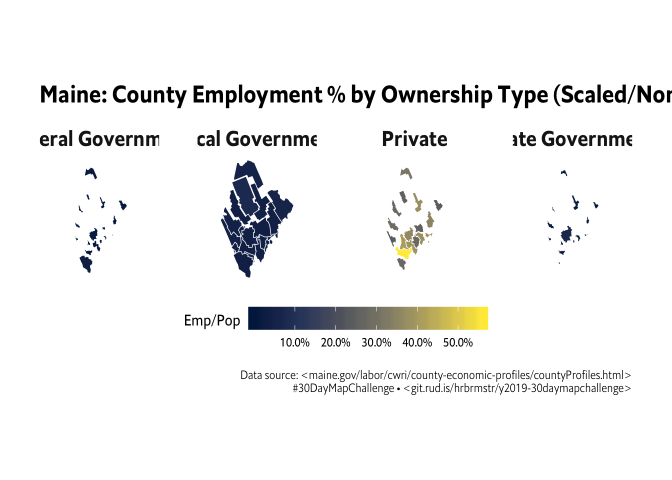
distinct(emp, ownership) %>%
  pull(ownership) %>%
  map(~{
    left_join(me_counties, filter(emp, ownership == .x), "NAME") %>%
      cartogram_ncont("emp_pop")
  }) %>%
  do.call(rbind, .) %>%
  ggplot() +
  geom_sf(aes(fill = emp_pop), color = "white", size = 0.25) +
  scale_x_continuous(expand = c(0, 100000)) +
  scale_fill_viridis_c(
    name = "Emp/Pop\n", label=scales::percent, option = "cividis", direction = 1
  ) +
  coord_sf(crs = albersusa::us_laea_proj, datum=NA) +
  facet_wrap(~ownership, ncol=4) +
  labs(
    title = "Maine: County Employment % by Ownership Type (Scaled/Non-contiguous)",
    caption = "Data source: <maine.gov/labor/cwri/county-economic-profiles/countyProfiles.html>\n#30DayMapChallenge • <git.rud.is/hrbrmstr/y2019-30daymapchallenge>"
  ) +
  theme_ipsum_es(grid="", strip_text_family = font_es_bold, strip_text_size = 16) +
  theme(strip.text = element_text(hjust = 0.5)) +
  theme(legend.position = "bottom") +
  theme(legend.key.width = unit(2.5, "lines"))
read_excel(here::here("data/county-profiles.xlsx"), "Poverty") %>%
janitor::clean_names() %>%
filter(
geography == "County"
) %>%
select(NAME = area_name, subject, percent) %>%
mutate(NAME = stri_replace_last_fixed(NAME, " Cty", "")) %>%
filter(subject %in% c(
"Under 18 years", "All people"
)) -> me_poverty
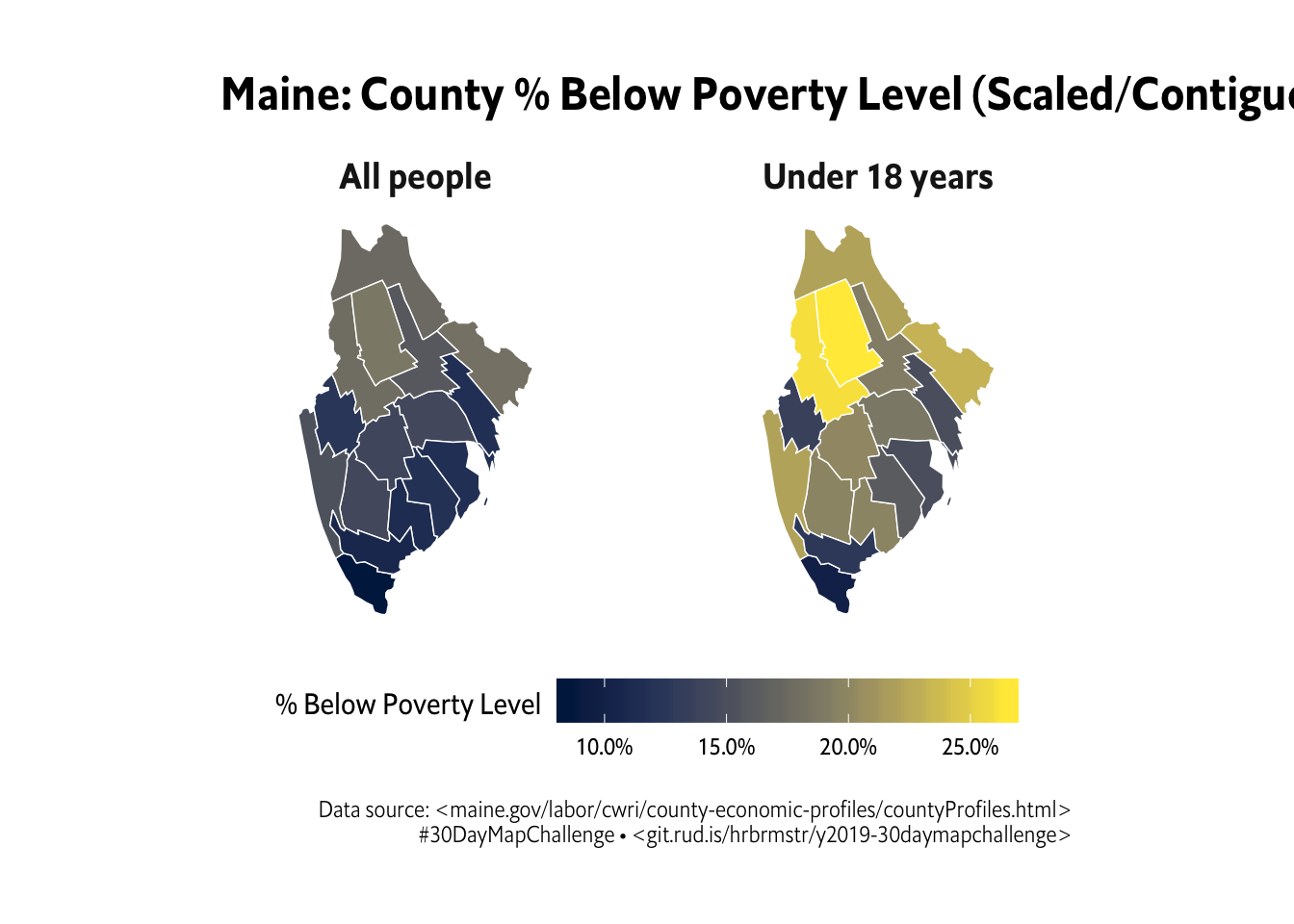
distinct(me_poverty, subject) %>%
pull(subject) %>%
map(~{
left_join(me_counties, filter(me_poverty, subject == .x), "NAME") %>%
cartogram_cont("percent")
}) %>%
do.call(rbind, .) %>%
ggplot() +
geom_sf(aes(fill = percent), color = "white", size = 0.25) +
scale_x_continuous(expand = c(0, 100000)) +
scale_fill_viridis_c(
name = "% Below Poverty Level\n", label=scales::percent, option = "cividis", direction = 1
) +
coord_sf(crs = albersusa::us_laea_proj, datum=NA) +
facet_wrap(~subject, ncol=4) +
labs(
title = "Maine: County % Below Poverty Level (Scaled/Contiguous)",
caption = "Data source: <maine.gov/labor/cwri/county-economic-profiles/countyProfiles.html>\n#30DayMapChallenge • <git.rud.is/hrbrmstr/y2019-30daymapchallenge>"
) +
theme_ipsum_es(grid="", strip_text_family = font_es_bold, strip_text_size = 14) +
theme(strip.text = element_text(hjust = 0.5)) +
theme(legend.position = "bottom") +
theme(legend.key.width = unit(2.5, "lines"))
distinct(me_poverty, subject) %>%
  pull(subject) %>%
  map(~{
    left_join(me_counties, filter(me_poverty, subject == .x), "NAME") %>%
      cartogram_ncont("percent")
  }) %>%
  do.call(rbind, .) %>%
  ggplot() +
  geom_sf(aes(fill = percent), color = "white", size = 0.25) +
  scale_x_continuous(expand = c(0, 100000)) +
  scale_fill_viridis_c(
    name = "% Below Poverty Level\n", label=scales::percent, option = "cividis", direction = 1
  ) +
  coord_sf(crs = albersusa::us_laea_proj, datum=NA) +
  facet_wrap(~subject, ncol=4) +
  labs(
    title = "Maine: County % Below Poverty Level (Scaled/Non-contiguous)",
    caption = "Data source: <maine.gov/labor/cwri/county-economic-profiles/countyProfiles.html>\n#30DayMapChallenge • <git.rud.is/hrbrmstr/y2019-30daymapchallenge>"
  ) +
  theme_ipsum_es(grid="", strip_text_family = font_es_bold, strip_text_size = 14) +
  theme(strip.text = element_text(hjust = 0.5)) +
  theme(legend.position = "bottom") +
  theme(legend.key.width = unit(2.5, "lines"))
