4 Day 2: Lines

4.1 Technologies/Techniques

R Simple Features {sf} manipulation, including making our own {sf} objects and turning {sf} objects into data frames
Acquiring basemaps from {rnaturalearth}
Using {ggplot2} geom_sf() to draw a map and geom_curve() to draw curved lines on it

4.2 Data Source: State Exports from Maine

The U.S. Census provides data on top exports from U.S. states. I came across the data they have on Maine²² and thought it’d be fun to use lines to show movement of goods outside of Maine.

My original attempt at this used {rvest} to scrape the HTML from the Census site. Then, whilst making this tome, I noticed the link at the bottom of the page for a mostly-clean CSV file²³ of the data, so we’ll use that for this example.

library(sf)
library(grid)
library(gridExtra)
library(rnaturalearth)
library(hrbrthemes)
library(tidyverse)

Before we get the data we need to bring in the base map we’ll be using since we’re going to need the geometries for it right after we process the data. We’ll be using the {rnaturalearth} package²⁴ in many subsequent challenges as it provides convenient access to a plethora of world regions.

We’ll use ne_countries() to grab all the countries at a larger scale as we do not need the detailed coastlines for a zoomed-out map, then ensure it’s giving us back a tidy {sf} object, then remove icky Antarctica²⁵ since it just takes up space and Maine sends no products there.

ne_countries(scale = "medium", returnclass = "sf") %>%
  filter(name != "Antarctica") -> world

glimpse(world)
## Observations: 240
## Variables: 64
## $ scalerank  <int> 3, 1, 1, 1, 1, 3, 3, 1, 1, 1, 3, 5, 3, 1, 1, 1, 1, 1, 1, 1…
## $ featurecla <chr> "Admin-0 country", "Admin-0 country", "Admin-0 country", "…
## $ labelrank  <dbl> 5, 3, 3, 6, 6, 6, 6, 4, 2, 6, 4, 5, 6, 6, 2, 4, 5, 6, 2, 5…
## $ sovereignt <chr> "Netherlands", "Afghanistan", "Angola", "United Kingdom", …
## $ sov_a3     <chr> "NL1", "AFG", "AGO", "GB1", "ALB", "FI1", "AND", "ARE", "A…
## $ adm0_dif   <dbl> 1, 0, 0, 1, 0, 1, 0, 0, 0, 0, 1, 1, 1, 0, 1, 0, 0, 0, 0, 0…
## $ level      <dbl> 2, 2, 2, 2, 2, 2, 2, 2, 2, 2, 2, 2, 2, 2, 2, 2, 2, 2, 2, 2…
## $ type       <chr> "Country", "Sovereign country", "Sovereign country", "Depe…
## $ admin      <chr> "Aruba", "Afghanistan", "Angola", "Anguilla", "Albania", "…
## $ adm0_a3    <chr> "ABW", "AFG", "AGO", "AIA", "ALB", "ALD", "AND", "ARE", "A…
## $ geou_dif   <dbl> 0, 0, 0, 0, 0, 0, 0, 0, 0, 0, 0, 0, 0, 0, 0, 0, 0, 0, 0, 0…
## $ geounit    <chr> "Aruba", "Afghanistan", "Angola", "Anguilla", "Albania", "…
## $ gu_a3      <chr> "ABW", "AFG", "AGO", "AIA", "ALB", "ALD", "AND", "ARE", "A…
## $ su_dif     <dbl> 0, 0, 0, 0, 0, 0, 0, 0, 0, 0, 0, 0, 0, 0, 0, 0, 0, 0, 0, 0…
## $ subunit    <chr> "Aruba", "Afghanistan", "Angola", "Anguilla", "Albania", "…
## $ su_a3      <chr> "ABW", "AFG", "AGO", "AIA", "ALB", "ALD", "AND", "ARE", "A…
## $ brk_diff   <dbl> 0, 0, 0, 0, 0, 0, 0, 0, 0, 0, 0, 0, 0, 0, 0, 0, 0, 0, 0, 0…
## $ name       <chr> "Aruba", "Afghanistan", "Angola", "Anguilla", "Albania", "…
## $ name_long  <chr> "Aruba", "Afghanistan", "Angola", "Anguilla", "Albania", "…
## $ brk_a3     <chr> "ABW", "AFG", "AGO", "AIA", "ALB", "ALD", "AND", "ARE", "A…
## $ brk_name   <chr> "Aruba", "Afghanistan", "Angola", "Anguilla", "Albania", "…
## $ brk_group  <chr> NA, NA, NA, NA, NA, NA, NA, NA, NA, NA, NA, NA, NA, NA, NA…
## $ abbrev     <chr> "Aruba", "Afg.", "Ang.", "Ang.", "Alb.", "Aland", "And.", …
## $ postal     <chr> "AW", "AF", "AO", "AI", "AL", "AI", "AND", "AE", "AR", "AR…
## $ formal_en  <chr> "Aruba", "Islamic State of Afghanistan", "People's Republi…
## $ formal_fr  <chr> NA, NA, NA, NA, NA, NA, NA, NA, NA, NA, NA, NA, NA, NA, NA…
## $ note_adm0  <chr> "Neth.", NA, NA, "U.K.", NA, "Fin.", NA, NA, NA, NA, "U.S.…
## $ note_brk   <chr> NA, NA, NA, NA, NA, NA, NA, NA, NA, NA, NA, NA, NA, NA, NA…
## $ name_sort  <chr> "Aruba", "Afghanistan", "Angola", "Anguilla", "Albania", "…
## $ name_alt   <chr> NA, NA, NA, NA, NA, NA, NA, NA, NA, NA, NA, NA, NA, NA, NA…
## $ mapcolor7  <dbl> 4, 5, 3, 6, 1, 4, 1, 2, 3, 3, 4, 1, 7, 2, 1, 3, 1, 2, 3, 1…
## $ mapcolor8  <dbl> 2, 6, 2, 6, 4, 1, 4, 1, 1, 1, 5, 2, 5, 2, 2, 1, 6, 2, 2, 2…
## $ mapcolor9  <dbl> 2, 8, 6, 6, 1, 4, 1, 3, 3, 2, 1, 2, 9, 5, 2, 3, 5, 5, 1, 2…
## $ mapcolor13 <dbl> 9, 7, 1, 3, 6, 6, 8, 3, 13, 10, 1, 7, 11, 5, 7, 4, 8, 8, 8…
## $ pop_est    <dbl> 103065, 28400000, 12799293, 14436, 3639453, 27153, 83888, …
## $ gdp_md_est <dbl> 2258.0, 22270.0, 110300.0, 108.9, 21810.0, 1563.0, 3660.0,…
## $ pop_year   <dbl> NA, NA, NA, NA, NA, NA, NA, NA, NA, NA, NA, NA, NA, NA, NA…
## $ lastcensus <dbl> 2010, 1979, 1970, NA, 2001, NA, 1989, 2010, 2010, 2001, 20…
## $ gdp_year   <dbl> NA, NA, NA, NA, NA, NA, NA, NA, NA, NA, NA, NA, NA, NA, NA…
## $ economy    <chr> "6. Developing region", "7. Least developed region", "7. L…
## $ income_grp <chr> "2. High income: nonOECD", "5. Low income", "3. Upper midd…
## $ wikipedia  <dbl> NA, NA, NA, NA, NA, NA, NA, NA, NA, NA, NA, NA, NA, NA, NA…
## $ fips_10    <chr> NA, NA, NA, NA, NA, NA, NA, NA, NA, NA, NA, NA, NA, NA, NA…
## $ iso_a2     <chr> "AW", "AF", "AO", "AI", "AL", "AX", "AD", "AE", "AR", "AM"…
## $ iso_a3     <chr> "ABW", "AFG", "AGO", "AIA", "ALB", "ALA", "AND", "ARE", "A…
## $ iso_n3     <chr> "533", "004", "024", "660", "008", "248", "020", "784", "0…
## $ un_a3      <chr> "533", "004", "024", "660", "008", "248", "020", "784", "0…
## $ wb_a2      <chr> "AW", "AF", "AO", NA, "AL", NA, "AD", "AE", "AR", "AM", "A…
## $ wb_a3      <chr> "ABW", "AFG", "AGO", NA, "ALB", NA, "ADO", "ARE", "ARG", "…
## $ woe_id     <dbl> NA, NA, NA, NA, NA, NA, NA, NA, NA, NA, NA, NA, NA, NA, NA…
## $ adm0_a3_is <chr> "ABW", "AFG", "AGO", "AIA", "ALB", "ALA", "AND", "ARE", "A…
## $ adm0_a3_us <chr> "ABW", "AFG", "AGO", "AIA", "ALB", "ALD", "AND", "ARE", "A…
## $ adm0_a3_un <dbl> NA, NA, NA, NA, NA, NA, NA, NA, NA, NA, NA, NA, NA, NA, NA…
## $ adm0_a3_wb <dbl> NA, NA, NA, NA, NA, NA, NA, NA, NA, NA, NA, NA, NA, NA, NA…
## $ continent  <chr> "North America", "Asia", "Africa", "North America", "Europ…
## $ region_un  <chr> "Americas", "Asia", "Africa", "Americas", "Europe", "Europ…
## $ subregion  <chr> "Caribbean", "Southern Asia", "Middle Africa", "Caribbean"…
## $ region_wb  <chr> "Latin America & Caribbean", "South Asia", "Sub-Saharan Af…
## $ name_len   <dbl> 5, 11, 6, 8, 7, 5, 7, 20, 9, 7, 14, 23, 22, 17, 9, 7, 10, …
## $ long_len   <dbl> 5, 11, 6, 8, 7, 13, 7, 20, 9, 7, 14, 27, 35, 19, 9, 7, 10,…
## $ abbrev_len <dbl> 5, 4, 4, 4, 4, 5, 4, 6, 4, 4, 9, 7, 10, 6, 4, 5, 4, 4, 5, …
## $ tiny       <dbl> 4, NA, NA, NA, NA, 5, 5, NA, NA, NA, 3, NA, 2, 4, NA, NA, …
## $ homepart   <dbl> NA, 1, 1, NA, 1, NA, 1, 1, 1, 1, NA, NA, NA, 1, 1, 1, 1, 1…
## $ geometry   <MULTIPOLYGON [°]> MULTIPOLYGON (((-69.89912 1..., MULTIPOLYGON …

We’re also going to need the coordinates for the center of Maine. There are many, many ways to get this, but we’ll use the built-in state data in R and convert it into an {sf} object along with transforming it to the the relatively new equal earth projection²⁶ since that will be the projection used in the final map. While the equal earth projection represents countries with equal-area throughout, it has other useful features (these are from the aforelinked resource):

An overall shape similar to that of the Robinson projection. (The Robinson, although popular and pleasing to the eye, is not equal-area as is the Equal Earth projection).
The curved sides of the projection suggest the spherical form of Earth.
Straight parallels that make it easier to compare how far north or south places are from the equator.
Meridians are evenly spaced along any given line of latitude.

me <- which(state.abb == "ME")

c(state.center$x[me], state.center$y[me]) %>% 
  st_point() %>% 
  st_sfc() %>%
  st_set_crs("+proj=longlat +datum=WGS84 +no_defs") %>%
  st_transform(crs = "+proj=eqearth +wktext") -> maine_center 

glimpse(maine_center)
## sfc_POINT of length 1; first list element:  'XY' num [1:2] -5643416 5533042

The data file has some explanatory header lines we need to skip.

if (!file.exists(here::here("data/exctyme.csv"))) {
  download.file(
    url = "https://www.census.gov/foreign-trade/statistics/state/data/exctyme.csv",
    destfile = here::here("data/exctyme.csv")
  )
}

cols(
  rank = col_character(),
  countryd = col_character(),
  val2015 = col_double(),
  val2016 = col_double(),
  val2017 = col_double(),
  val2018 = col_double(),
  share15 = col_double(),
  share16 = col_double(),
  share17 = col_double(),
  share18 = col_double(),
  change = col_double()
) -> export_cols

read_csv(
  file = here::here("data/exctyme.csv"), skip = 4,
  col_types = export_cols
) %>% 
  select(country = countryd, val2018) %>% 
  filter(!(country %in% c("World", "Top 25"))) %>% 
  mutate(country = case_when( # clean up the countries since they need to match what's in the natural earth shapefile
    country == "Macau" ~ "Macao",
    country == "Korea, South" ~ "Korea",
    TRUE ~ country
  )) %>%
  arrange(desc(val2018)) %>%
  slice(1:20) %>% # top 20 only to avoid clutter
  left_join(world, by = c("country" = "name")) %>% # get the geometries for the target countries so we can get their centers
  mutate(to = suppressWarnings(st_centroid(geometry)) %>% st_transform(crs = "+proj=eqearth +wktext")) %>% # need to transform (see note below)
  select(country, val2018, to) %>%
  mutate(maine = maine_center) -> xdf # temporary variable

glimpse(xdf)
## Observations: 20
## Variables: 4
## $ country <chr> "Canada", "China", "Malaysia", "Italy", "Japan", "Korea", "Ge…
## $ val2018 <dbl> 1427.51, 204.53, 121.93, 87.46, 87.24, 66.81, 66.02, 60.28, 5…
## $ to      <POINT [m]> POINT (-7006259 7039606), POINT (9003565 4532178), POIN…
## $ maine   <POINT [m]> POINT (-5643416 5533042), POINT (-5643416 5533042), POI…

4.3 Arrows of Commerce

We’re going to use geom_curve() since it will intelligently place the curves with arrows for us, but we need to have the points in a plain ol’ data frame since it’s not an {sf} geom.

st_coordinates(xdf$maine) %>%
  as_tibble() %>%
  set_names(c("from_x", "from_y")) %>%
  bind_cols(
    st_coordinates(xdf$to) %>%
      as_tibble() %>%
      set_names(c("to_x", "to_y")),
    select(xdf, country, val2018)
  ) -> maine_exports_to

glimpse(maine_exports_to)
## Observations: 20
## Variables: 6
## $ from_x  <dbl> -5643416, -5643416, -5643416, -5643416, -5643416, -5643416, -…
## $ from_y  <dbl> 5533042, 5533042, 5533042, 5533042, 5533042, 5533042, 5533042…
## $ to_x    <dbl> -7006259.5, 9003564.5, 10498125.3, 1007217.2, 11900282.5, 110…
## $ to_y    <dbl> 7039606.1, 4532178.3, 486773.1, 5229390.2, 4649786.8, 4511945…
## $ country <chr> "Canada", "China", "Malaysia", "Italy", "Japan", "Korea", "Ge…
## $ val2018 <dbl> 1427.51, 204.53, 121.93, 87.46, 87.24, 66.81, 66.02, 60.28, 5…

4.4 Turning the Tables

Adding a table to the map for some more detailed annotation layer seemed like it might be a good idea after looking at the map without it. We’ll use the tableGrob() function from the {gridExtra} to make an object we can place on the ggplot2 plot object like we would any other annotation object.

as_tibble(maine_exports_to) %>%
  select(Country = country, Exports = val2018) %>%
  mutate(Exports = glue::glue("{scales::comma(Exports)}M USD")) %>%
  tableGrob(
    rows = NULL,
    theme = ttheme_default(
      core = list(
        fg_params = list(
          fontfamily = font_rc,
          hjust = c(rep(0, 20), rep(1, 20)),
          x = c(rep(0.1, 20), rep(0.9, 20))
        )
      )
    )
  ) -> tabl

glimpse(tabl)
## gtable, containing 
## grobs (84) : chr [1:84] "text[GRID.text.91]" "text[GRID.text.92]" "rect[GRID.rect.93]" ...
## layout :
## 'data.frame':    84 obs. of  7 variables:
##  $ t   : num  1 1 1 1 2 3 4 5 6 7 ...
##  $ l   : num  1 2 1 2 1 1 1 1 1 1 ...
##  $ b   : num  1 1 1 1 2 3 4 5 6 7 ...
##  $ r   : num  1 2 1 2 1 1 1 1 1 1 ...
##  $ z   : num  1 2 0 0 1 2 3 4 5 6 ...
##  $ clip: chr  "on" "on" "on" "on" ...
##  $ name: chr  "colhead-fg" "colhead-fg" "colhead-bg" "colhead-bg" ...
## widths :
## unit vector of length 2 
## heights :
## unit vector of length 21 
## respect :
##  logi FALSE
## rownames :
##  chr [1:21] "r1" "r2" "r3" "r4" "r5" "r6" "r7" "r8" "r9" "r10" "r11" "r12" ...
## name :
##  chr "colhead-fg"
## gp :
##  NULL
## vp :
##  NULL

4.5 Drawing the Map

ggplot() +
  geom_sf(data = world, size = 0.125, fill = "#3B454A", color = "#b2b2b2") +
  geom_curve(
    data = maine_exports_to, aes(x = from_x, y = from_y, xend = to_x, yend = to_y, color = val2018, size = val2018),
    curvature = 0.2, arrow = arrow(length = unit(10, "pt"), type = "closed"),
  ) +
  guides(
    color = guide_legend(reverse = TRUE)
  ) +
  annotation_custom(tabl, xmin = -16920565, xmax = -14000000,  ymin=761378/2.25, ymax = 761378) + # values are in eqarea meters
  coord_sf(crs = "+proj=eqearth +wktext") +
  scale_color_distiller(
    palette = "RdYlBu", trans = "log10", name = "(Size & color\nlog10 scale)", label = scales::comma,
    breaks = c(30, 50, 100, 300, 1000), limits = c(15, 1500)
  ) +
  scale_size_continuous(
    trans = "log10", range = c(0.75, 3),
    breaks = c(30, 50, 100, 300, 1000), limits = c(15, 1500),
    guide = FALSE
  ) +
  theme_ft_rc(grid="") +
  labs(
    x = NULL, y = NULL,
    title = "Top 20 (by Value) Export Destinations for Maine Goods (2018)",
    caption = "Data source: Census Bureau Foreign Trade <www.census.gov/foreign-trade/statistics/state/data/me.html>\n#30DayMapChallenge"
  ) +
  theme_ft_rc(grid="") +
  theme(legend.key.height = unit(2.8, "lines")) +
  theme(legend.position = c(0.2, 0.3)) +
  theme(axis.text.x = element_blank())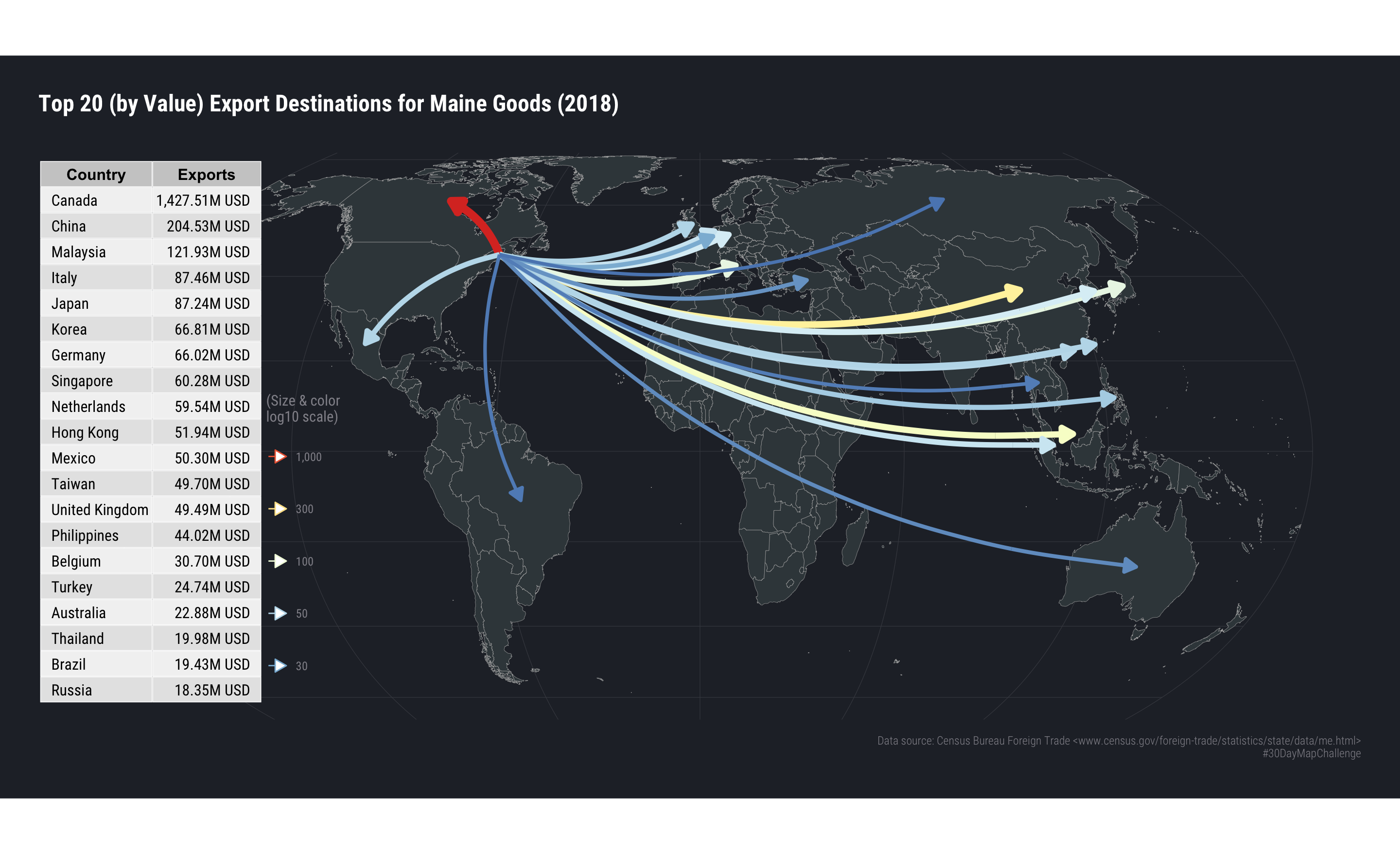

4.6 In Review

This exercise used “fancier” annotations and showed how to mix in more traditional {ggplot2} geoms with geom_sf().

4.7 Try This At Home

We used “+proj=eqearth +wktext” for the map projection. Try changing it to other global map projections and see what you need to do to make the annotations work.

The annotation table could use some attention. Explore the customization possibilities with ttheme_default() and consider removing the redundant M USD in each row and putting that info in the table header.