13 Day 11: Elevation

13.1 Technologies/Techniques

Working with R Simple Features {sf}
Dealing with multiple-sourced shapefiles
Using {ggplot2} geom_sf() to heavily stylize a map

13.2 Data Source: Maine Elevation Contours

We love Acadia National Park⁴⁷ and I used today’s challenge to finally chart out all of Mount Desert Island⁴⁸ (MDI). There are links in the code-blocks to the various data sources where I obtained basemaps and elevation data. Where possible, these elements have been carved up and minified to make it easier to work with them.

library(sf)
library(hrbrthemes)
library(tidyverse)

The first bit retrieves all of the towns that make up MDI since I could not find a single MDI shapefile (I really should make one after this exercise). We do this work primarily to get the outline of the island so we can use that to extract the elevation data and lake data for that region from two other shapefiles. This is very straightforward in the {sf} ecosystem (it “feels” just like working with plain ol’ tidy data frames).

if (!all(file.exists(here::here("data", c("mdi.rds", "mdi-border.rds", "mdi-inland-water.rds"))))) {

  # http://hub.arcgis.com/datasets/c7fdfaabcffa480c820e8be4a19bb298/data?layer=3

  # get all the towns and focus on the ones we care about
  st_read(here::here("data/Maine_Boundaries_Town_Polygon/Maine_Boundaries_Town_Polygon.shp")) %>%
    filter(TOWN %in% c("Bar Harbor", "Mount Desert", "Tremont", "Southwest Harbor", "Cranberry Isles")) %>%
    select(OBJECTID) %>%
    filter( # this removes island and meta-borders we don't want
      OBJECTID < 3000,
      !OBJECTID %in% c(2412, 2519, 2480, 2520, 2530, 2533, 2523, 2266, 2661, 2694, 2255, 2287, 2631, 2674, 2643, 2698)
    ) %>%
    st_union() -> mdi_border # finally, smush them all together

  # the actual elevation contours
  st_read(here::here("data/Shape/Elev_Contour.shp")) %>%
    st_crop(xmin = -68.4719, ymin = 44.2108, xmax = -68.1542, ymax = 44.4666) %>% # reduce scope for faster intersection
    st_transform(26919) %>%
    st_intersection(mdi_border) -> mdi # only what's in the smushed outline above

  # lakes and ponds
  
  # "http://easterndivision.s3.amazonaws.com/Freshwater/LakeData.zip"
  
  st_read(here::here("data/lake-data/lakepolys.shp")) %>%
    filter(STATE_ABBR == "ME") %>% # reduce scope for faster intersection
    st_transform(26919) %>%
    st_intersection(mdi_border) %>% # only what's in the smushed outline above
    filter(!is.na(GNIS_NAME)) -> inland_water # finally, get rid of unnamed water bodies

  # save ^^ work out so we don't have to do it again
  saveRDS(mdi, here::here("data/mdi.rds"))
  saveRDS(mdi_border, here::here("data/mdi-border.rds"))
  saveRDS(inland_water, here::here("data/mdi-inland-water.rds"))

}

# read in our hard work
mdi <- readRDS(here::here("data/mdi.rds"))
mdi_border <- readRDS(here::here("data/mdi-border.rds"))
inland_water <- readRDS(here::here("data/mdi-inland-water.rds"))

Here’s the border we made:

plot(mdi_border)

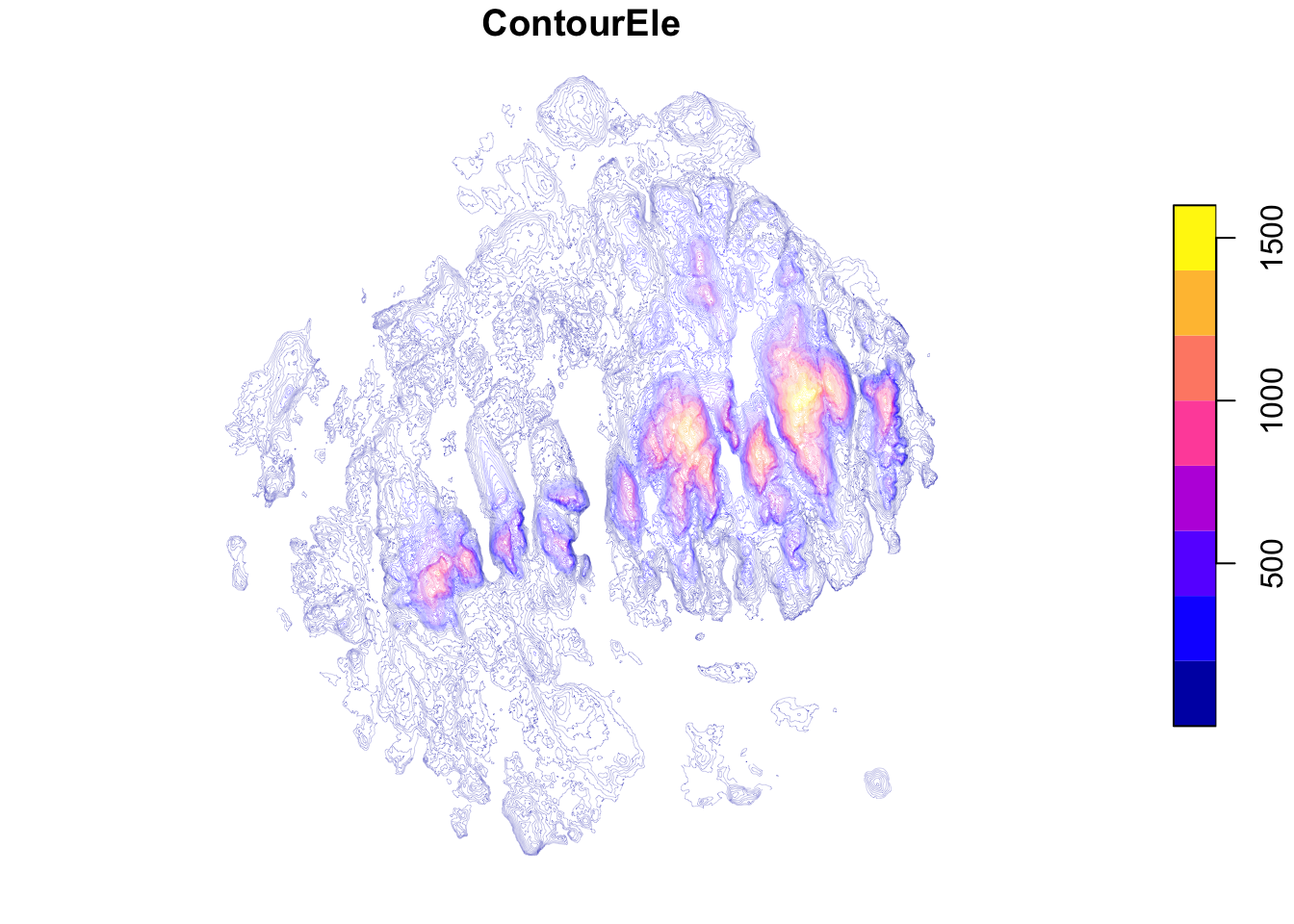
Here’s the elevation contours:

plot(mdi["ContourEle"], lwd=0.1)

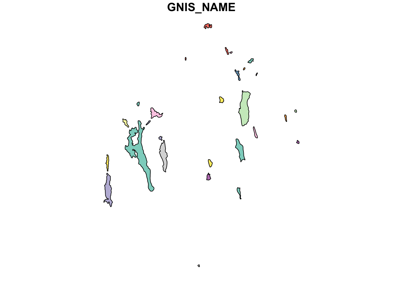
Here are bodies of water on the island:

plot(inland_water["GNIS_NAME"])

We’re going to make our own {sf} points geometry object so we can add an annotation layer for some of the mountains on the final map. One key item to note is ensuring we use the same coordinate reference system (CRS) for this outer_lab object as we have for the other shapefiles we’ve mangled.

tibble(
  lat = c(44.3380, 44.3526, 44.3351, 44.3426, 44.3329),
  lng = c(-68.3119, -68.2251, -68.2438, -68.2728, -68.2667),
  size = c(4.5, 3, 3, 3, 3),
  angle = c(-80, 0, 0, 0, 0),
  lab = c("Somes Sound", "Cadillac\nMountain", "Pemetic\nMountain", "Sargent\nMountain", "Penobscot\nMountain")
) %>%
  st_as_sf(coords = c("lng", "lat"), crs = 4326) %>%
  st_transform(26919) -> outer_lab

13.3 Drawing the Map

Don’t let this final map fool you. I spent quite a bit of time tweaking aesthetics to get it to this point and I think it still could use a bit of work.

We use the inland_water object twice, once to plot the polygons and the second time to label certain lakes/ponds.

ggplot() +
  geom_sf(data = mdi_border, color = "#999999", fill = NA, size = 2, alpha = 1/20) + # water light outline
  geom_sf(data = mdi_border, color = "black", fill = "#f6e3b9", size = 0.5) + # maine border
  geom_sf(data = mdi, aes(color = ContourEle), size = 0.1) + # the contours
  geom_sf(data = inland_water, color = "black", fill = "#3a4f5b", size = 0.3) + # the lakes and ponds
  geom_sf_text( # label inland water we care about
    data = inland_water %>%
      filter(
        GNIS_NAME %in% c("Jordan Pond", "Eagle Lake", "Echo Lake", "Seal Cove Pond") |
          (GNIS_NAME == "Long Pond" & ACRES > 100)
      ),
    aes(label = GNIS_NAME),
    family = font_es, color = "white",
    size = c(3.25, 3.25, 2.5, 2.5, 2.5),  # these align with the ordered factor names
    angle = c(87.5, -75, -75, -80, -87.5)
  ) +
  geom_sf_text(
    data = outer_lab,
    aes(label = lab, size = I(size)+0.125, angle = I(angle)),
    family = font_es, color = c("black", "white", "white", "white", "white"), lineheight = 0.875
  ) +
  geom_sf_text(
    data = outer_lab,
    aes(label = lab, size = I(size), angle = I(angle)),
    family = font_es, color = c("white", "black", "black", "black", "black"), lineheight = 0.875
  ) +
  scale_color_viridis_c(
    name = "Elevation (ft)", option = "magma", label = scales::comma
  ) +
  coord_sf(datum = NA) +
  labs(
    x = NULL, y = NULL,
    title = "Mount Desert Island / Acadia National Park Elevation Contours",
    caption = "Data source: ArcGIS/<maine.gov> • #30DayMapChallenge"
  ) +
  theme_ipsum_es(grid="", plot_title_size = 24) +
  theme(plot.background = element_rect(fill = "#3a4f5b", color = "#3a4f5b")) +
  theme(panel.background = element_rect(fill = "#3a4f5b", color = "#3a4f5b")) +
  theme(legend.title = element_text(color = "white")) +
  theme(legend.text = element_text(color = "white")) +
  theme(plot.title = element_text(hjust = 0.5, color = "white")) +
  theme(plot.caption = element_text(color = "white")) +
  theme(legend.position = c(0.9, 0.275))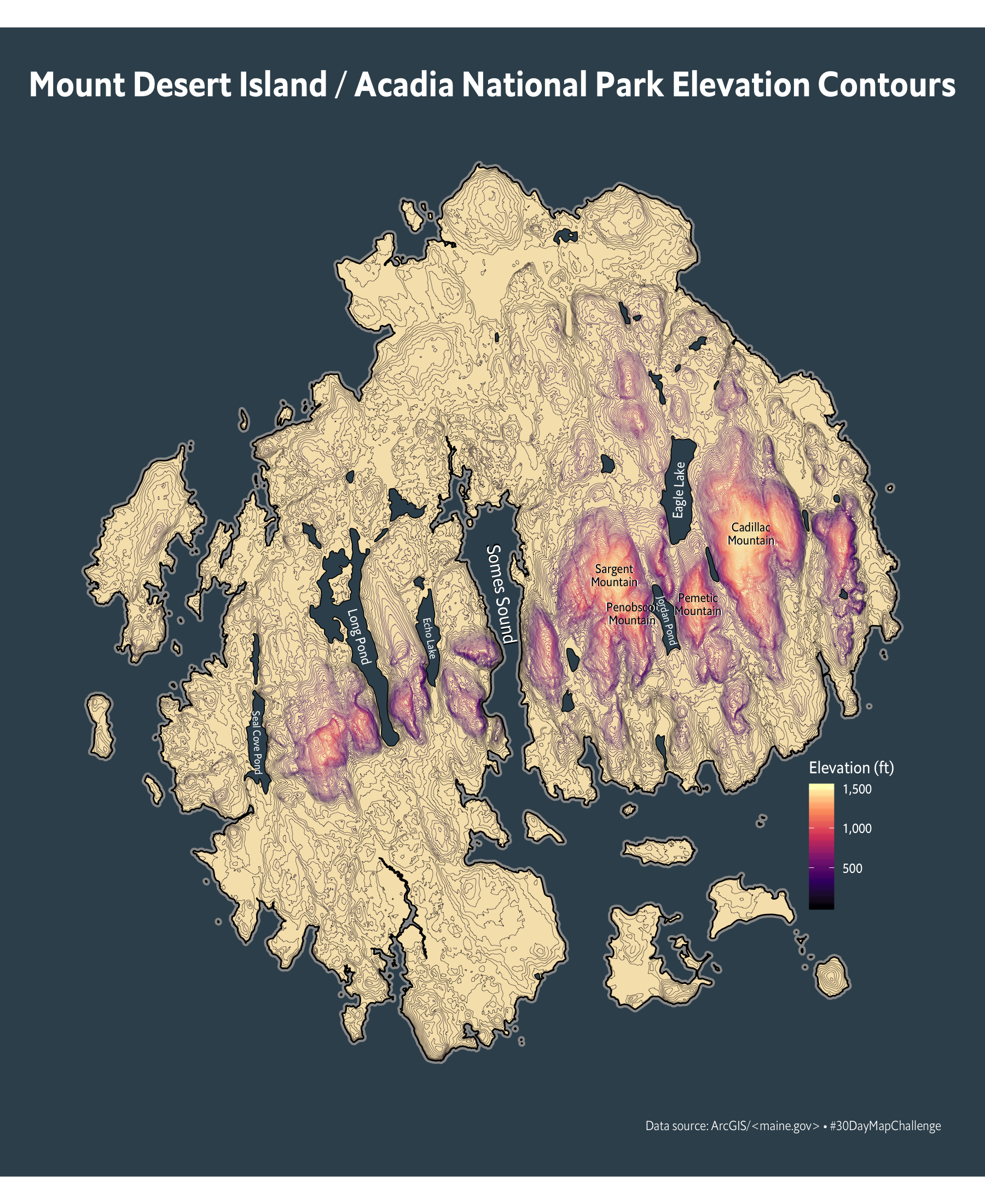

13.4 In Review

We pulled in shapefiles from multiple sources and did a bit of slicing and dicing on and with them. We also used {ggplot2} to build a highly stylized final map (vs some of the plain ones we’ve built thus far).

13.5 Try This At Home

Pick one of your favorite hiking, biking, fishing, (etc.) spots and start spelunking for shapefiles you can use to create a similar map. “Googling” for xyz elevation contours would be a good start for finding data you can use. Many states/towns are doing a great job providing GIS data these days, so your search should be fruitful and fairly brief.