16 Day 14: Tracks
16.1 Technologies/Techniques
- Working with R Simple Features
{sf} - Incorporating
{rnaturalearth}base layers - Using an external shapefile with temporal data layers
- Generating
{magick}animation frames with{ggplot2}andgeom_sf()
16.2 Data Source: Historical Railroad Transportation
I took “tracks” quite literally for today’s challenge and grabbed a shapefile that documents the creation and expansion of the conterminus U.S. railroad system. We’ll grab the data and generate animation frames as we’ve done in previous challenges.
This data collection is from Jeremy Atack’s “Historical Geographic Information Systems (GIS) database of U.S. Railroads (May 2016)52.
if (!file.exists(here::here("data/RR1826-1911Modified0509161.zip"))) {
download.file(
url = "https://cdn.vanderbilt.edu/vu-my/wp-content/uploads/sites/133/2019/04/14090344/RR1826-1911Modified0509161.zip",
destfile = here::here("data/RR1826-1911Modified0509161.zip")
)
unzip(
zipfile = here::here("data/RR1826-1911Modified0509161.zip"),
exdir = here::here("data/RR1826-1911Modified0509161")
)
}
r1 <- st_read(here::here("data/RR1826-1911Modified0509161/RR1826-1911Modified050916.shp"))
## Reading layer `RR1826-1911Modified050916' from data source `/Users/hrbrmstr/books/30-day-map-challenge/data/RR1826-1911Modified0509161/RR1826-1911Modified050916.shp' using driver `ESRI Shapefile'
## Simple feature collection with 78832 features and 8 fields
## geometry type: MULTILINESTRING
## dimension: XY
## bbox: xmin: -2332623 ymin: -1329179 xmax: 2252703 ymax: 1558942
## epsg (SRID): 102003
## proj4string: +proj=aea +lat_1=29.5 +lat_2=45.5 +lat_0=37.5 +lon_0=-96 +x_0=0 +y_0=0 +datum=NAD83 +units=m +no_defs
glimpse(r1)
## Observations: 78,832
## Variables: 9
## $ track <dbl> 0.0921356, 0.6290380, 0.0368666, 0.1132930, 1.5171500, 0.27…
## $ VxCount <int> 4, 5, 2, 2, 3, 6, 13, 8, 2, 2, 38, 4, 2, 9, 12, 4, 2, 5, 10…
## $ Gauge <dbl> 51.0, 51.0, 56.5, 56.5, 56.5, 56.5, 56.5, 56.5, 56.5, 56.5,…
## $ RRname <fct> Delaware & Hudson, Delaware & Hudson, Baltimore and Ohio, B…
## $ InOpBy <int> 1830, 1830, 1830, 1830, 1872, 1872, 1872, 1972, 1972, 1972,…
## $ ExactDate <int> 1829, 1829, 1830, 1830, 0, 0, 0, 0, 0, 0, 0, 1830, 1830, 18…
## $ FIDAll <dbl> 0, 1, 2, 3, 4, 5, 6, 7, 8, 9, 10, 11, 12, 13, 14, 15, 16, 1…
## $ Edited <dbl> 0, 0, 0, 0, 0, 0, 0, 0, 0, 0, 0, 0, 0, 0, 0, 0, 0, 0, 0, 0,…
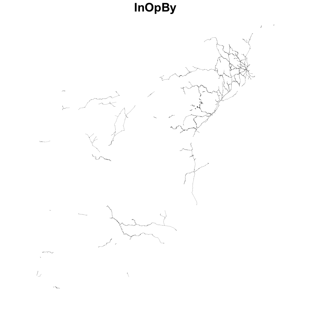
## $ geometry <MULTILINESTRING [m]> MULTILINESTRING ((1703095 6..., MULTILINEST…We can use base plot() to take a look at railroad development up through 1850:
For the final animation layers We’ll need a basemap and we’ll also make a thicker border for this map:
16.3 Drawing the Map
To make each layer for our final animation we’ll iterate over each unique year and then draw the base layer border, the state borders and then all the railroad tracks up until the current iteration year. We’ll stitch them all together with {magick}.
NOTE: This animation generation takes a while (5-15m depending on your system).
in_op_rng <- sort(unique(r1$InOpBy))

img <- image_graph(width=1000*2, height=600*2, res=96)

pb <- progress_estimated(length(in_op_rng))

for (i in in_op_rng) {

  pb$tick()$print()

  ggplot() +
    geom_sf(data = border, color = "#252525", size = 1, fill = NA) +
    geom_sf(data = states, color = "#b2b2b2", size = 0.1, fill = "white", linetype = "dotted") +
    geom_sf(data = filter(r1, InOpBy <= i), aes(color = InOpBy), size = 0.1) +
    coord_sf(crs = albersusa::us_laea_proj, datum = NA) +
    scale_color_continuous(limits = range(r1$InOpBy)) +
    labs(
      x = NULL, y = NULL,
      title = sprintf("U.S. Railroad Expansion • Year: %s", i),
      subtitle = "The 'Ties' That Bound Us Together",
      caption = "Data source: <my.vanderbilt.edu/jeremyatack/data-downloads/>\nhttps://git.rud.is/hrbrmstr/y2019-30daymapchallenge • #30DayMapChallenge"
    ) +
    theme_ipsum_es(grid="") +
    theme(plot.title = element_text(hjust = 0.5)) +
    theme(plot.subtitle = element_text(hjust = 0.5)) +
    theme(panel.background = element_rect(fill = "#b15928")) +
    theme(legend.position = "none") -> gg

  print(gg)

}

dev.off()

img <- image_animate(img)

image_write(img, here::here("img/rr.gif"))
16.4 In Review
More animations this time, but with a cumulative, temporal aspect to them. We also worked with a pretty neat shapefile that documents history with the GIS information.
16.5 Try This At Home
Try working with different colors and line sizes depending on the track types.
Use the extra metadata in the downloaded GIS file as tooltip fodder in a {mapdeck} version of the tracks.