7 Day 5: Raster

7.1 Technologies/Techniques

Using {sf} and {stars} together
Working with GeoTIFF files
Using {ggplot2} geom_sf() to draw basemaps and rasters together
Making animated maps with {magick}

7.2 Data Source: U.S. Minimum Daily Temperature Rasters

The U.S. National Weather Service’s Climate Prediction Center maintains many datasets³⁵ and I thought it’d be neat to make an animation of the daily minimum temperatures across the conterminus U.S. for 2019.

The data files are GeoTIFF³⁶ files. They store values in a grid format (kinda like the grid we made in the previous challenge). You can store multiple “layers” (bands) in a raster images like this but the NWS CPC stores them in individual files.

Here’s what one of the images looks like:

library(sf)
library(httr)
library(stars)
library(glue)
library(stringi)
library(magick)
library(rnaturalearth)
library(hrbrthemes)
library(tidyverse)

tf <- tempfile(fileext = ".tif")

download.file("ftp://ftp.cpc.ncep.noaa.gov/GIS/GRADS_GIS/GeoTIFF/TEMP/us_tmin/us.tmin_nohads_ll_20191130_float.tif", tf)

tmpstars <- read_stars(tf) 

unlink(tf)

tmpstars
## stars object with 2 dimensions and 1 attribute
## attribute(s):
##  file11ef8201f9f45.tif 
##  Min.   :-22.81403     
##  1st Qu.: -1.35325     
##  Median :  0.00000     
##  Mean   :  0.06779     
##  3rd Qu.:  0.28419     
##  Max.   : 22.52072     
## dimension(s):
##   from  to  offset delta                       refsys point values    
## x    1 141 -130.25   0.5 +proj=longlat +datum=WGS8... FALSE   NULL [x]
## y    1  71   55.25  -0.5 +proj=longlat +datum=WGS8... FALSE   NULL [y]

plot(tmpstars)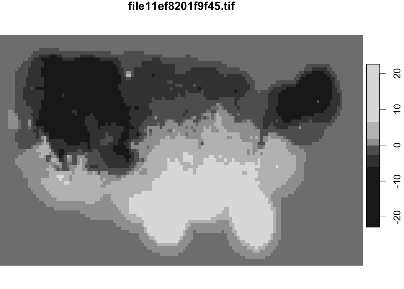

We’re going to want to clean these up a bit and mask/crop the raster to the conterminus borders, plus re-project them to a proper CRS. But, first we need to get the data and that means downloading a few hundred files. Thankfully, they’re small so this will be fairly quick.

httr::GET(
  url = "ftp://ftp.cpc.ncep.noaa.gov/GIS/GRADS_GIS/GeoTIFF/TEMP/us_tmin/"
) -> res

rawToChar(res$content) %>% 
  stri_split_lines() %>% 
  unlist() %>% 
  keep(stri_detect_fixed, "ll_2019") %>% 
  stri_replace_first_regex("^[^us]*", "") %>% 
  walk(~{
    if (!file.exists(here::here(glue("data/temps{.x}"))))
    download.file(
      url = glue("ftp://ftp.cpc.ncep.noaa.gov/GIS/GRADS_GIS/GeoTIFF/TEMP/us_tmin/{.x}"),
      destfile = here::here(glue("data/temps/{.x}"))
    )
  })

We could have used download.file()’s ability to download files in parallel, but it’s very likely that for ~300 files it would have consumed all available sockets on your system (it’s not a very intelligent function).

We’ll use these files in a bit.

7.3 Getting the Base Layer

We’ll use the ne_states() function to grab the U.S. and remove Alaska & Hawaii. We’ll make another, projected copy of it for use later on and also dissolve all the state borders with st_union() in yet-another copy.

# lower 48 borders
ne_states("united states of america", returnclass = "sf") %>%
  filter(!(postal %in% c("AK", "HI"))) -> states 

states_proj <- st_transform(states, "+proj=laea +lat_0=45 +lon_0=-100 +x_0=0 +y_0=0 +a=6370997 +b=6370997 +units=m +no_defs")
# lower 48 big poly
whole <- st_union(states)

7.4 Reading in Rasters

We’ll use the {stars} package to work on these rasters. Unfortunately, some of the GeoTIFF files are corrupt so we’ll have to wrap the reading operation with {purrr}’s possibly() function to avoid abrupt stops.

Believe it or not, the following block of code is super fast thanks to {stars}.

# some of the rasters have errors
safe_stars <- possibly(read_stars, NULL, quiet = TRUE)

# read them in, discarding problematic ones
list.files(here::here("data/temps"), full.names = TRUE) %>%
  purrr::map(safe_stars) %>%
  discard(is.null) -> temp_stars

Each raster is ultimately a matrix of values. We’re going to want to keep a consistent color scale range for all the plots so we’ll need to get the range for all of the rasters. This, too, is wicked fast:

temp_stars %>%
  purrr::map(~range(.x[[1]])) %>%
  purrr::flatten_dbl() %>%
  range() -> min_max # get min/max values

min_max
## [1] -40.39574  32.76227

7.5 Drawing the Map

You may recall that we have multiple versions of the U.S. state polygons. We first crop the rasters with the un-projected, dissolved state border, then project the raster to the equal area projection we’ll be using and convert it to an {sf} object for plotting.

We also need to extract the date from the filename, which is preserved in the {stars} object.

We’re wrapping all this into a {magick} idiom so we can easily turn each image into an animated gif frame.

frames <- image_graph(700, 600, res = 96)

purrr::walk(temp_stars, ~{

  temps <- .x
  st_crop(temps, whole) %>% 
    st_transform("+proj=laea +lat_0=45 +lon_0=-100 +x_0=0 +y_0=0 +a=6370997 +b=6370997 +units=m +no_defs") %>% 
    st_as_sf() %>% 
    select(val=1, geometry) -> temps

  temp_date <- as.Date(stri_match_first_regex(names(.x), "([[:digit:]]{8})")[,2], format = "%Y%m%d")

  ggplot() +
    geom_sf(data = temps, aes(fill = val, color = val)) +
    geom_sf(data = states_proj, fill = NA, color = "white", size = 0.125) +
    scale_fill_viridis_c(
      option = "magma", limits = c(-40, 35), breaks = c(-40, -20, 0, 20, 35)
    ) +
    scale_color_viridis_c(
      option = "magma", limits = c(-40, 35), breaks = c(-40, -20, 0, 20, 35)
    ) +
    coord_sf(datum = NA) +
    guides(
      fill = guide_colourbar(title.position = "top"),
      color = guide_colourbar(title.position = "top")
    ) +
    labs(
      x = NULL, y = NULL,
      color = "Min temp range for 2019 (°C)",
      fill = "Min temp range for 2019 (°C)",
      title = glue::glue("Minimum Temps for {temp_date}")
    ) +
    theme_ft_rc(grid="") +
    theme(plot.title = element_text(hjust = 0.5)) +
    theme(axis.text = element_blank()) +
    theme(legend.key.width = unit(2, "lines")) +
    theme(legend.position = "bottom") -> gg

  print(gg)

})

dev.off

gif <- image_animate(frames, fps = 5)

# save it out

image_write(gif, here::here("out/temps.gif"))

7.6 In Review

This challenge introduced the {stars} package which makes using raster day speedy, efficient, and fun! We combined that with previous knowledge of how to make other types of maps and used our {magick} powers to spin animation gold from straw data.

7.7 Try This At Home

Try doing the same process for the maximum temperature raster files and then poke at the {stars} st_warp() function and see if you can resample the grid into a finer-grained (or coarser) grid.