10 Day 8: Green

10.1 Technologies/Techniques

R Simple Features {sf}
Working with GeoJSON files
Using geo-data from the {tigris} package
Using {ggplot2} geom_sf() to draw lines
Using {mapdeck} and {sf} to draw lines in an interactive map

10.2 Data Source: U.S. TIGER Roads

The U.S. Census Bureau maintains many databases of geographic information free for use by anyone. The data is referenced as “Topologically Integrated Geographic Encoding and Referencing” — i.e. “TIGER” — and they describe land attributes such as roads, buildings, rivers, and lakes, along with census tracts. I thought it’d be fun to map all the roads in Maine with “green” in the name.

The {tigris} package³⁹ makes accessing TIGER data pretty darned easy. So easy, in fact, that we’re going to use both {ggplot2} and {mapdeck}⁴⁰ just to introduce another cool mapping package.

To use the {mapdeck} bits, you’ll have to head on over to mapbox⁴¹ and register for a free account and get a mapbox API token and put it into an environment variable named MAPBOX_PUBLIC_TOKEN which you can put in your ~/.Renviron file⁴².

library(sf)
library(tigris)
library(stringi)
library(hrbrthemes)
library(mapdeck)
library(tidyverse)

mapdeck_api_key <- Sys.getenv("MAPBOX_PUBLIC_TOKEN") # since we're going to use it later on

st_read(here::here("data/me-counties.json")) %>% # get the Maine shapefile
  st_set_crs(4326) -> maine
## Reading layer `cb_2015_maine_county_20m' from data source `/Users/hrbrmstr/books/30-day-map-challenge/data/me-counties.json' using driver `TopoJSON'
## Simple feature collection with 16 features and 10 fields
## geometry type:  MULTIPOLYGON
## dimension:      XY
## bbox:           xmin: -71.08434 ymin: 43.05975 xmax: -66.9502 ymax: 47.45684
## epsg (SRID):    NA
## proj4string:    NA

The list_counties() function in {tigris} will let us iterate over county names to pull the roads for each county using the roads() function. You are encouraged to use the options(tigris_use_cache=TRUE) feature of {tigris} to avoid re-downloading data (i.e. save bandwidth). By default, {tigris} operations return old-school R spatial objects, so we also have to ask it to give us an {sf} object back.

list_counties("me") %>%
  pull(county) %>%
  map(~roads("me", .x, class="sf")) -> me_roads

glimpse(me_roads[[1]])
## Observations: 4,963
## Variables: 5
## $ LINEARID <chr> "110190956609", "1106087305718", "110190956357", "1101909576…
## $ FULLNAME <chr> "Memorial Brg Rmp", "Mason St Exd", "Glendale Ave Exd", "Bow…
## $ RTTYP    <chr> "M", "M", "M", "M", "M", "M", "M", "M", "M", "M", "M", "M", …
## $ MTFCC    <chr> "S1400", "S1400", "S1400", "S1400", "S1400", "S1400", "S1400…
## $ geometry <LINESTRING [°]> LINESTRING (-70.20493 44.11..., LINESTRING (-70.2…

Now, we’ll go through each {sf} object and keep only roads with “green” in the name and combine the {sf} objects into one (note the use of rbind() vs bind_rows()):

map(me_roads, ~filter(.x, stri_detect_fixed(FULLNAME, "green", case_insensitive = TRUE))) %>%
  do.call(rbind, .) -> green_roads

glimpse(green_roads)
## Observations: 514
## Variables: 5
## $ LINEARID <chr> "1103672634386", "110190951882", "1102205002980", "110190953…
## $ FULLNAME <chr> "Green Ave", "Green St", "Evergreen Ln", "Greene St", "Everg…
## $ RTTYP    <chr> "M", "M", "M", "M", "M", "M", "M", "M", "M", "M", "M", "M", …
## $ MTFCC    <chr> "S1400", "S1400", "S1400", "S1400", "S1400", "S1400", "S1400…
## $ geometry <LINESTRING [°]> LINESTRING (-70.1743 44.460..., LINESTRING (-70.2…

10.3 Drawing the Map (Part 1)

For the {ggplot2} version, we just use very familiar geom_sf() plotting idioms:

ggplot() +
  geom_sf(data = maine, color = "#b2b2b2", size = 0.125, fill = "#3B454A") +
  geom_sf(data = green_roads, color = "forestgreen", size = 0.75) +
  coord_sf(datum = NA) +
  labs(
    title = "The 'Green' Roads of Maine",
    subtitle = "Linestrings of all roads in Maine with 'green' in the name",
    caption = "Data source: {tigris} • #30DayMapChallenge"
  ) +
  theme_ft_rc() +
  theme(plot.title = element_text(hjust = 0.5)) +
  theme(plot.subtitle = element_text(hjust = 0.5)) +
  theme(axis.text = element_blank()) +
  theme(legend.position = "none")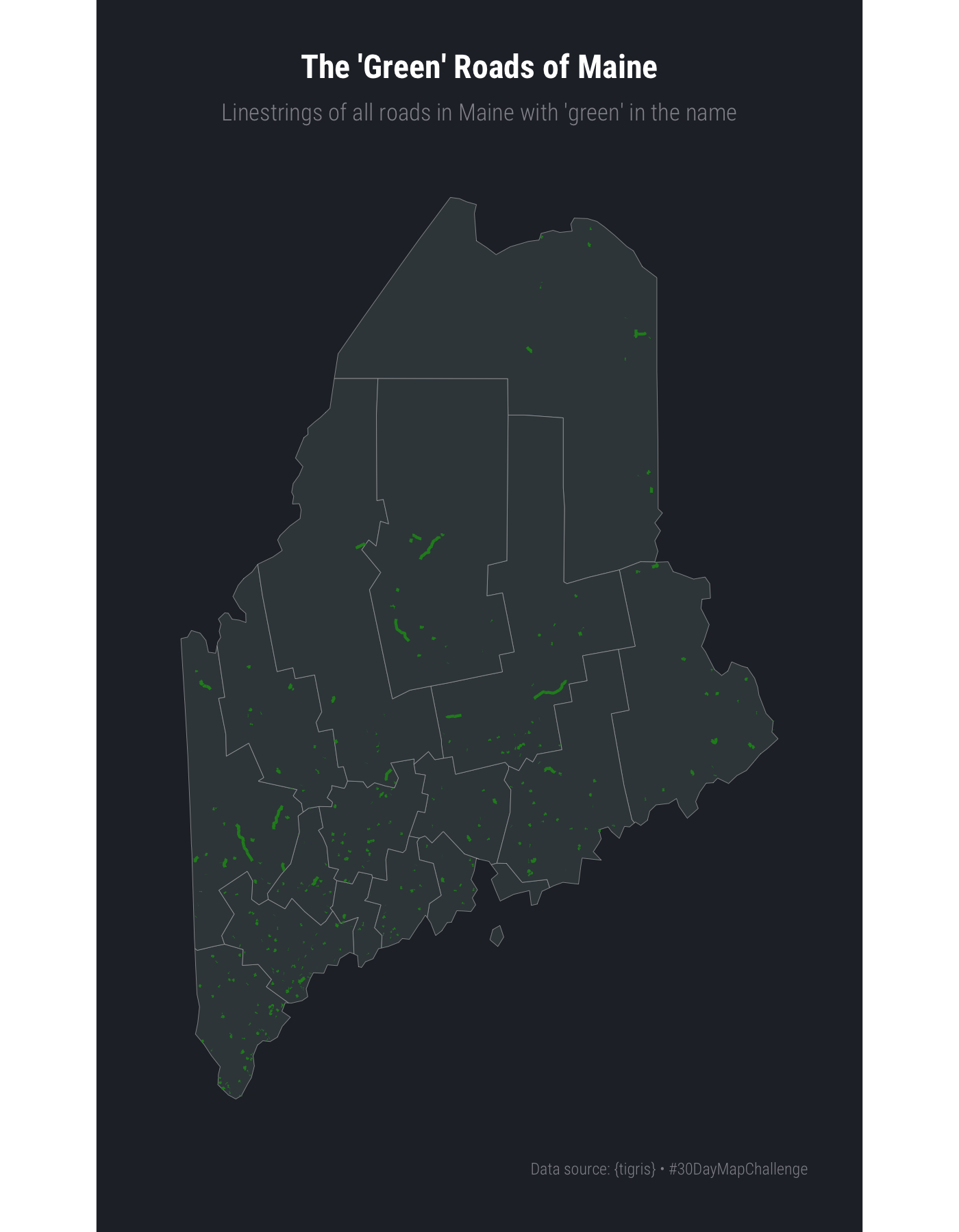

10.4 Drawing the Map (Part 2)

The {mapdeck} version is even easier. We first setup the map style, starting location, and zoom level, then add in a layer of our {sf} green roads and ask {mapdeck} to use the FULLNAME of the road as a tooltip, so when you zoom in and hover you’ll see what the actual road name is.

We also use update_view = FALSE to avoid any update to the map position after the linestrings have been drawn.

mapdeck(
  token = mapdeck_api_key,
  style = mapdeck_style("dark"),
  location = c(-69.4455, 45.2538),
  zoom = 6
) %>%
  add_sf(
    data = green_roads,
    layer_id = "FULLNAME",
    stroke_width = 2,
    stroke_colour = "#228b22",
    tooltip = "FULLNAME",
    update_view = FALSE
  ) %>%
  add_title("The 'Green' Roads of Maine")

10.5 In Review

This challenged introduced online, interactive mapping with {mapdeck} as well as the {tigris} package. These are two powerful R packages that dramatically reduce friction when building maps with R. The {mapdeck} package is especially useful when you have many elements to map since {ggplot2} can be slow when there are many features to draw and {mapdeck} uses OpenGL to speedily render features using your GPU.

10.6 Try This At Home

Try using {mapdeck} and {tigris} to map all the towns in the conterminus U.S. with “green” in their name.