3 Day 1: Points

3.1 Technologies/Techniques

R Simple Features {sf} manipulation
Using {ggplot2} geom_sf() to plot points on a map
Making faceted maps

3.2 Data Source: K-12 Ransomware Incidents

The topic for Day 1 was “points” and I opted to use a Google spreadsheet of (mostly) geolocated U.S. K-12 school ransomware incidents¹⁴ going back to 2016 as a base for plotting locations of these events on a map. This checked the “cyber” and “United States” requirements boxes in my list of constraints and also helped ease into the challenge (it doesn’t get much more basic than points on a map, though we are mixing it up a bit with facets).

Since not all the detailed addresses were geolocated I decided to use the Geocodio service¹⁵ via my {rgeocodio} package¹⁶ to geocode down to the city/state level.

library(sf)
library(rgeocodio)
library(albersusa)
library(hrbrthemes)
library(googlesheets4)
library(ggthemes)
library(tidyverse)

To access the Google spreadsheet we’re using the {googlesheets4} package¹⁷ and you would do well to read through the overview¹⁸ if you’re not familiar with it.

Below, we’re:

accessing the sheet via the sheet ID
making a year_public variable so we can facet by year
thinning out the data frame to just the year and address

read_sheet("https://docs.google.com/spreadsheets/d/1p-_GRo4YPW7m4QnjvErKD4U67t8-O6aDBlRjy9V8g8Y/edit?usp=sharing") %>% 
  mutate(
    year_public = ifelse(
      year_public < 2000, lubridate::year(date_added), year_public
    ) %>% factor()
  ) %>% 
  select(year_public, city_st) -> xdf

glimpse(xdf)
## Observations: 690
## Variables: 2
## $ year_public <fct> 2016, 2016, 2016, 2016, 2016, 2016, 2016, 2016, 2016, 201…
## $ city_st     <chr> "Corpus Christi, TX", "Chesapeake, VA", "Baton Rouge, LA"…

3.3 Geocoding Points

We’ll now geolocate the records using the Geocodio service. To do that, you’ll need a free API key¹⁹ stored in a GEOCODIO_API_KEY environment variable. The ~/.Renviron file²⁰ is a good place to put this setting.

The Geocodio service has a very generous free tier but that doesn’t mean we shouldn’t cache API results, so we’ll make sure to do that after the geocoding is finished.

if (!file.exists(here::here("data/2019-11-01-geocoded.rds"))) {
  coded <- gio_batch_geocode(xdf$city_st)
  saveRDS(coded, here::here("data/2019-11-01-geocoded.rds"))
}

coded <- readRDS(here::here("data/2019-11-01-geocoded.rds"))

glimpse(coded)
## Observations: 690
## Variables: 17
## $ query             <chr> "Corpus Christi, TX", "Chesapeake, VA", "Baton Roug…
## $ response_results  <list> [<data.frame[80 x 11]>, <data.frame[14 x 11]>, <da…
## $ response_warnings <list> ["There is a newer API version available, please c…
## $ formatted_address <chr> "Corpus Christi, TX", "Chesapeake, VA", "Baton Roug…
## $ city              <chr> "Corpus Christi", "Chesapeake", "Baton Rouge", "Kat…
## $ state             <chr> "TX", "VA", "LA", "TX", "OH", "IL", "WA", "NY", "TX…
## $ country           <chr> "US", "US", "US", "US", "US", "US", "US", "US", "US…
## $ street            <chr> NA, NA, NA, NA, NA, NA, NA, NA, NA, NA, NA, NA, NA,…
## $ suffix            <chr> NA, NA, NA, NA, NA, NA, NA, NA, NA, NA, NA, NA, NA,…
## $ zip               <chr> NA, NA, NA, NA, NA, NA, NA, NA, NA, NA, NA, NA, NA,…
## $ number            <chr> NA, NA, NA, NA, NA, NA, NA, NA, NA, NA, NA, NA, NA,…
## $ postdirectional   <chr> NA, NA, NA, NA, NA, NA, NA, NA, NA, NA, NA, NA, NA,…
## $ formatted_street  <chr> NA, NA, NA, NA, NA, NA, NA, NA, NA, NA, NA, NA, NA,…
## $ predirectional    <chr> NA, NA, NA, NA, NA, NA, NA, NA, NA, NA, NA, NA, NA,…
## $ secondaryunit     <chr> NA, NA, NA, NA, NA, NA, NA, NA, NA, NA, NA, NA, NA,…
## $ prefix            <chr> NA, NA, NA, NA, NA, NA, NA, NA, NA, NA, NA, NA, NA,…
## $ secondarynumber   <chr> NA, NA, NA, NA, NA, NA, NA, NA, NA, NA, NA, NA, NA,…

The Geocodio service often retuns multiple response_results records for each geolocation since the geolocation process is often fraught with peril (or errors/uncertainty).

glimpse(coded$response_results[[1]])
## Observations: 80
## Variables: 11
## $ formatted_address          <chr> "Corpus Christi, TX 78401", "Corpus Christ…
## $ accuracy                   <dbl> 1, 1, 1, 1, 1, 1, 1, 1, 1, 1, 1, 1, 1, 1, …
## $ accuracy_type              <chr> "place", "place", "place", "place", "place…
## $ source                     <chr> "TIGER/Line® dataset from the US Census Bu…
## $ address_components.city    <chr> "Corpus Christi", "Corpus Christi", "Corpu…
## $ address_components.county  <chr> "Nueces County", "Nueces County", "Nueces …
## $ address_components.state   <chr> "TX", "TX", "TX", "TX", "TX", "TX", "TX", …
## $ address_components.zip     <chr> "78401", "78472", "78463", "78465", "78466…
## $ address_components.country <chr> "US", "US", "US", "US", "US", "US", "US", …
## $ location.lat               <dbl> 27.79780, 27.74022, 27.77700, 27.77700, 27…
## $ location.lng               <dbl> -97.39907, -97.57921, -97.46321, -97.46321…

We’ll go with the first geocoding result for each entry since they’re ordered from most confident to least confident.

bind_cols(
  xdf,
  select(coded, r = response_results, state) %>% 
    mutate(r = map(r, ~.x[1,])) %>% 
    unnest(r) %>% 
    select(state, lng = location.lng, lat = location.lat) 
) %>% 
  filter(!is.na(lat), !is.na(lng)) -> xdf

glimpse(xdf)
## Observations: 687
## Variables: 5
## $ year_public <fct> 2016, 2016, 2016, 2016, 2016, 2016, 2016, 2016, 2016, 201…
## $ city_st     <chr> "Corpus Christi, TX", "Chesapeake, VA", "Baton Rouge, LA"…
## $ state       <chr> "TX", "VA", "LA", "TX", "OH", "IL", "WA", "NY", "TX", "FL…
## $ lng         <dbl> -97.39907, -76.21876, -91.18561, -95.73376, -83.07613, -9…
## $ lat         <dbl> 27.79780, 36.74999, 30.44924, 29.83756, 40.02311, 40.8044…

3.4 Making a Simple Features Object

Now we have longitude/latitude pairs to work with, but there’s a catch. We’re going to use the {albersusa} package²¹ since it has basemaps that tuck Alaska and Hawaii underneath the conterminous United States, so we’ll need to use the same elide formula for any geolocated Alaska or Hawaii points. Thankfully there’s a points_elided() function in {albersusa} to help us do just that.

We’ll also create what will ultimately become the facet labels and turn the whole data frame into an {sf} object so we can use geom_sf() to plot the data.

bind_cols(
  select(xdf, -lng, -lat),   # everythign but lng/lat
  select(xdf, lng, lat) %>%  # take out lng/lat
    points_elided() %>%      # elide them; since we gave it a data frame, they come back with the us_laea_proj CRS
    rename(lng = lon, lat = lat) # so we'll use that at the end of the pipe when we turn the data back into an {sf} object
) %>% 
  left_join(
    count(., year_public), by = "year_public"
  ) %>% 
  mutate(lab = glue::glue("{year_public} : {n} Tracked Incidents")) %>% 
  st_as_sf(coords = c("lng", "lat"), crs = us_laea_proj) -> incidents

glimpse(incidents)
## Observations: 687
## Variables: 6
## $ year_public <fct> 2016, 2016, 2016, 2016, 2016, 2016, 2016, 2016, 2016, 201…
## $ city_st     <chr> "Corpus Christi, TX", "Chesapeake, VA", "Baton Rouge, LA"…
## $ state       <chr> "TX", "VA", "LA", "TX", "OH", "IL", "WA", "NY", "TX", "FL…
## $ n           <int> 66, 66, 66, 66, 66, 66, 66, 66, 66, 66, 66, 66, 66, 66, 6…
## $ lab         <glue> "2016 : 66 Tracked Incidents", "2016 : 66 Tracked Incide…
## $ geometry    <POINT [m]> POINT (258699 -1901781), POINT (2089241 -616785.2),…

3.5 Drawing the Map

We’ll need a base map to plot the points on so let’s get that via the usa_sf() from {albersusa}.

usa <- usa_sf("laea")

Now, we’ll use a core geom_sf() plotting idiom by laying down a base map layer and then plotting the points layer. geom_sf() is smart enough to know to draw polygons when it sees that type of geometry in an {sf} object and the same for points, lines, etc.

We can use all the standard aesthetics we’re used to using with other {ggplot2} geoms. Here, we’ll use a dark map background and filled points, faceting by year.

ggplot() +
  geom_sf( # plot the base map
    data = usa, fill = "#3B454A", size = 0.125, color = "#b2b2b277"
  ) +
  geom_sf( # plot the points
    data = incidents, aes(fill = lab), 
    color = "white", size = 1.5, alpha = 2/3, shape = 21,
    show.legend = FALSE # no legend since we're using facets and it'd just be redundant
  ) + 
  scale_color_tableau() +
  coord_sf(datum = NA) + # using datum = NA turns off the graticule 
  facet_wrap(~lab) +
  labs(
    title = "Locations of K-12 Ransomware Incidents 2016-2019 (Sept)",
    caption = "2019 #30DayMapChallenge"
  ) +
  theme_ft_rc(grid="", strip_text_face = "bold") +
  theme(axis.text = element_blank()) +
  theme(strip.text = element_text(color = "white"))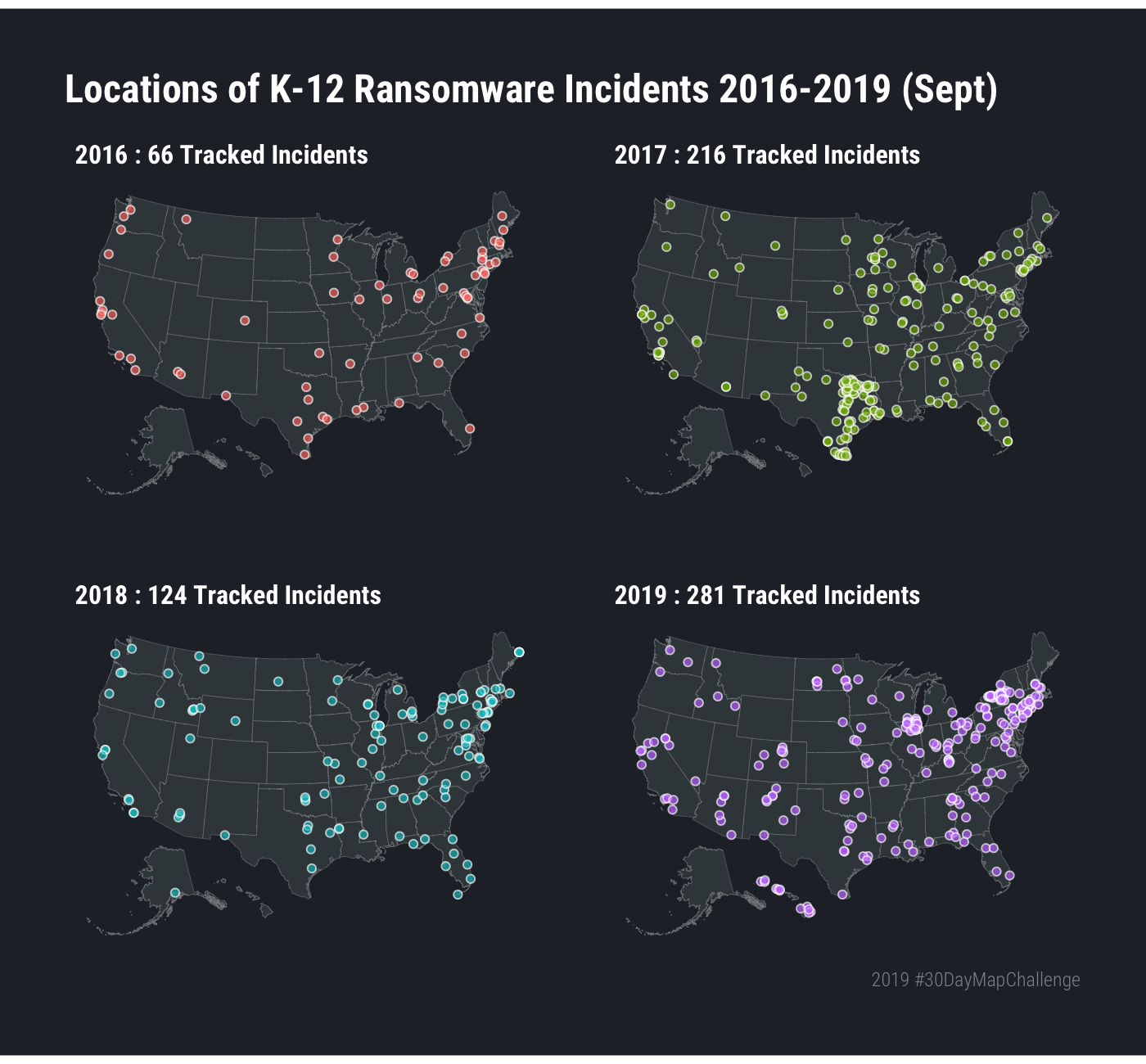

3.6 In Review

Most of the chapters in the book follow the same pattern of deciding on a data source, obtaining the data, and determining the way you want to communicate the results with a map. Most also follow the pattern of laying down a base {sf} map and adding layers.

3.7 Try This At Home

To get some practice with geom_sf() adaptability, use st_insersection() or the already geolocated state information to count incidents by year and state and switch the point-based map to a choropleth (filled state polygons).