12 Day 10: Black and White
12.1 Technologies/Techniques
- R Simple Features
{sf} - Working with
{tigris}data - Using
{ggplot2}geom_sf()to draw linestrings
12.2 Data Source: U.S. TIGER Roads
Since we’re already familiar with TIGER / {tigris} let’s use the entire roads data set for Maine to paint a picture of Maine without borders (i.e. let the roads make the map to see just how much of Maine we can recognize just with the primary road system).
First, we’ll build up the roads for all the Maine counties and save our work since it takes a few seconds to make the combined dataset:
if (!file.exists(here::here("data/me-roads.shp"))) {

  st_read(here::here("data/me-counties.json")) %>%
    st_set_crs(4326) -> maine

  list_counties("me") %>%
    pull(county) %>%
    map(~roads("me", .x, class="sf")) -> me_roads

  me_roads <- do.call(rbind, me_roads)

  st_write(me_roads, here::here("data/me-roads.shp"))

}

me_roads <- st_read(here::here("data/me-roads.shp"))
## Reading layer `me-roads' from data source `/Users/hrbrmstr/books/30-day-map-challenge/data/me-roads.shp' using driver `ESRI Shapefile'
## Simple feature collection with 156822 features and 4 fields
## geometry type:  LINESTRING
## dimension:      XY
## bbox:           xmin: -71.07829 ymin: 43.06587 xmax: -66.95202 ymax: 47.45985
## epsg (SRID):    NA
## proj4string:    +proj=longlat +ellps=GRS80 +no_defs

count(as_tibble(me_roads), RTTYP) # as_tibble() speeds this up quite a bit
## # A tibble: 7 x 2
##   RTTYP     n
##   <fct> <int>
## 1 C        15
## 2 I        35
## 3 M     81469
## 4 O      2629
## 5 S      1465
## 6 U       437
## 7 <NA>  70772
The RTTYP column is the "Route Type Code` and the abbreviated single letter description equates to the following types:
C: CountyI: InterstateM: Common NameO: OtherS: State recognizedU: U.S.
There are over 70,000 <NA> roads and we’ll choose not to plot them since we’re already going to be asking {ggplot2} to plot more than enough linestrings for us.
12.3 Drawing the Map
The only difference here is that we’re going to split out the state/county/interstate/main roads into separate {sf} objects since we’re going to be using different colors for the interstate roads to stylize them a bit more.
state <- filter(me_roads, RTTYP == "S")
county <- filter(me_roads, RTTYP == "C")
interstate <- filter(me_roads, RTTYP == "I")
main <- filter(me_roads, RTTYP == "M")

ggplot() +
  geom_sf(data = main, color = "#777777", size = 0.075, alpha = 2/3) +
  geom_sf(data = state, color = "#999999", size = 0.1, alpha = 1/2) +
  geom_sf(data = county, color = "#eeeeee", size = 0.125, alpha = 1/5) +
  geom_sf(data = interstate, color = "#999999", size = 2, alpha = 1/10) +
  geom_sf(data = interstate, color = "black", size = 1, alpha = 1/5) +
  geom_sf(data = interstate, color = "#aaaaaa", size = 1/2, alpha = 1/2) +
  labs(
    title = "Maine Without Borders",
    caption = "Data source: {tigris} • #30DayMapChallenge"
  ) +
  theme_ft_rc(grid="") +
  theme(plot.title = element_text(hjust = 0.5)) +
  theme(plot.background = element_rect(fill = "black", color = "black")) +
  theme(panel.background = element_rect(fill = "black", color = "black")) +
  theme(panel.grid = element_blank()) +
  theme(axis.ticks = element_blank()) +
  theme(axis.text = element_blank())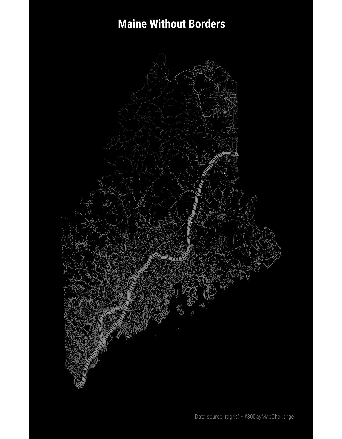
12.4 In Review
We did a bit more stylizing this time and also looked at the complete {tigris} roads data set for Maine. We also saw that {ggplot2} can process tens of thousands of linestrings pretty quickly!
12.5 Try This At Home
Add in the <NA> roads and focus a bit more on stylizing. Increase the plot size and resolution so the stylizing becomes even more vivid as folks zoom in.
Try repeating the idiom for a large city or different U.S. region.