21 Day 19: Urban
21.1 Technologies/Techniques
- Giving
{raster}some 💙 using GeoTIFF files - Working with
{tigris} - Using
{rnaturalearth}and{tigris}polygons and raster layers together - Combining
{sf}geom_sf()withgeom_tile()
21.2 Data Source: Black Marble (Light Pollution)
We live in rural Maine for many reasons, one of which is to have the privilege of being able to see more of the night sky than most city folk are able to view. This light pollution is tracked by NASA’s Black Marble59 project. In their own words:
At night, satellite images of Earth capture a uniquely human signal–artificial lighting. Remotely-sensed lights at night provide a new data source for improving our understanding of interactions between human systems and the environment. NASA has developed the Black Marble, a daily calibrated, corrected, and validated product suite, so nightlight data can be used effectively for scientific observations. Black Marble is playing a vital role in research on light pollution, illegal fishing, fires, disaster impacts and recovery, and human settlements and associated energy infrastructures.
I decided to compare known New England urban areas to the Black Marble data to both show that these areas do contribute to this light pollution and to see just where these centers of light pollution are located.
library(raster)
library(sf)
library(tigris)
library(hrbrthemes)
library(rnaturalearth)
library(tidyverse)
First we want a base layer of New England states so we just subset out our targets from the {rnaturalearth} shapefiles and created a border polygon at the same time to help with styling and more subsetting later on.
ne_states("United States of America", returnclass = "sf") %>%
  filter(
    name %in% c(
      "Maine", "New Hampshire", "Massachusetts", "Vermont", "New Jersey",
      "Connecticut", "New York", "Rhode Island", "Pennsylvania"
    )) -> neng

border <- st_union(neng)
Now we need the known urban areas from {tigris} which we’ll discover by retrieving the shapefile and then intersecting with our New England border:
urban_areas(cb = TRUE, class = "sf") %>%
  st_transform(st_crs(neng)) -> urban

neng_urban <- st_intersection(urban, border)
I hastily grabbed one of the Black Marble images from 2016 (we’ll come back to this in the “Try This at Home” section) and you should be aware that it’s a pretty large file if you’re interactively working through this challenge.
The NASA GeoTiFF is for the entire earth, but we just need New England, so we’re going to use {raster} functions (vs {stars} which we’ve used in other challenges) since it has been the workhorse when working with this type of data for a long time and you may come across older projects or even newer workflows that rely on it.
The concepts/idioms are very similar to {stars}, but without {sf} ecosystem compatibility. We’ll read in the Black Marble raster, reduce the amount of data we’re going to work with by masking it to the border polygon we made a little while ago, take that smaller raster area and project it to the CRS we’ll be using in the final map, then turn the entire raster into a data frame that we can use with geom_tile() to plot the light show.
The final data frame is much smaller than the starting raster and will plot very quickly in {ggplot2}.
if (!all(file.exists(here::here("data", c("BlackMarble_2016_3km_geo.tif", "bm-spdf.rds"))))) {

  download.file(
    url = "https://eoimages.gsfc.nasa.gov/images/imagerecords/144000/144898/BlackMarble_2016_3km_geo.tif",
    destfile = here::here("data/BlackMarble_2016_3km_geo.tif")
  )

  if (!file.exists(here::here("bm-spdf.rds"))) {

    bm <- raster(here::here("data/BlackMarble_2016_3km_geo.tif"))
    bm <- mask(bm, as(border, "Spatial"))
    bm <- projectRaster(bm, crs = crs(albersusa::us_laea_proj))
    bm <- mask(bm, as(st_transform(border, crs(albersusa::us_laea_proj)), "Spatial"))

    bm_spdf <- as.data.frame(as(bm, "SpatialPixelsDataFrame"))
    colnames(bm_spdf) <- c("value", "x", "y")

    saveRDS(bm_spdf, here::here("data/bm-spdf.rds"))
  }

}

bm_spdf <- readRDS(here::here("data/bm-spdf.rds"))

glimpse(bm_spdf)
## Observations: 151,102
## Variables: 3
## $ value <dbl> 33.541698, 26.729914, 25.000000, 25.000000, 25.000000, 12.08073…
## $ x     <dbl> 2311921, 2312894, 2313867, 2314840, 2315813, 2316786, 2307056, …
## $ y     <dbl> 732127.1, 732127.1, 732127.1, 732127.1, 732127.1, 732127.1, 729…
The value column is the brightness value at a given raster cell.
21.3 Drawing the Map
We’ll lay down the border polygon with a black fill, then tile out the brightness cells. We’ll put the urban areas polygons on top of that, then very light state outlines, followed by a lighter version of the border outline with no fill. I had to play a with with the colors and this isn’t necessarily the best final representation.
ggplot() +
  geom_sf(data = neng, fill = "black", color = "#2b2b2b", size = 0.125) +
  geom_tile(data = bm_spdf, aes(x, y, fill = value)) +
  geom_sf(data = neng_urban, fill = "#54278f55", color = "#54278f", size = 0.15) +
  geom_sf(data = neng, fill = NA, color = "#b2b2b2", size = 0.125) +
  geom_sf(data = border, fill = NA, color = "white", size = 1/4) +
  scale_fill_distiller(name = "Brightness", palette = "Greys") +
  coord_sf(crs = albersusa::us_laea_proj, datum = NA) +
  guides(fill = guide_colourbar(title.position = "top")) +
  labs(
    x = NULL, y = NULL,
    title = "In Blackest Night : How New England Urban Areas\nContribute To Light Pollution",
    subtitle = "Urban areas in purple with 33% alpha overlaid on top of\nNASA Earth Observatory 'Black Marble' Light Raster",
    caption = "Data: NASA <earthobservatory.nasa.gov/features/NightLights/page3.php>; {tigris} • #30DayMapChallenge"
  ) +
  theme_ft_rc(grid="") +
  theme(legend.position = c(0.3, 0.85)) +
  theme(legend.direction = "horizontal") +
  theme(legend.key.width = unit(1.5, "lines")) +
  theme(panel.background = element_rect(color = "#252a32", fill = "#252a32"))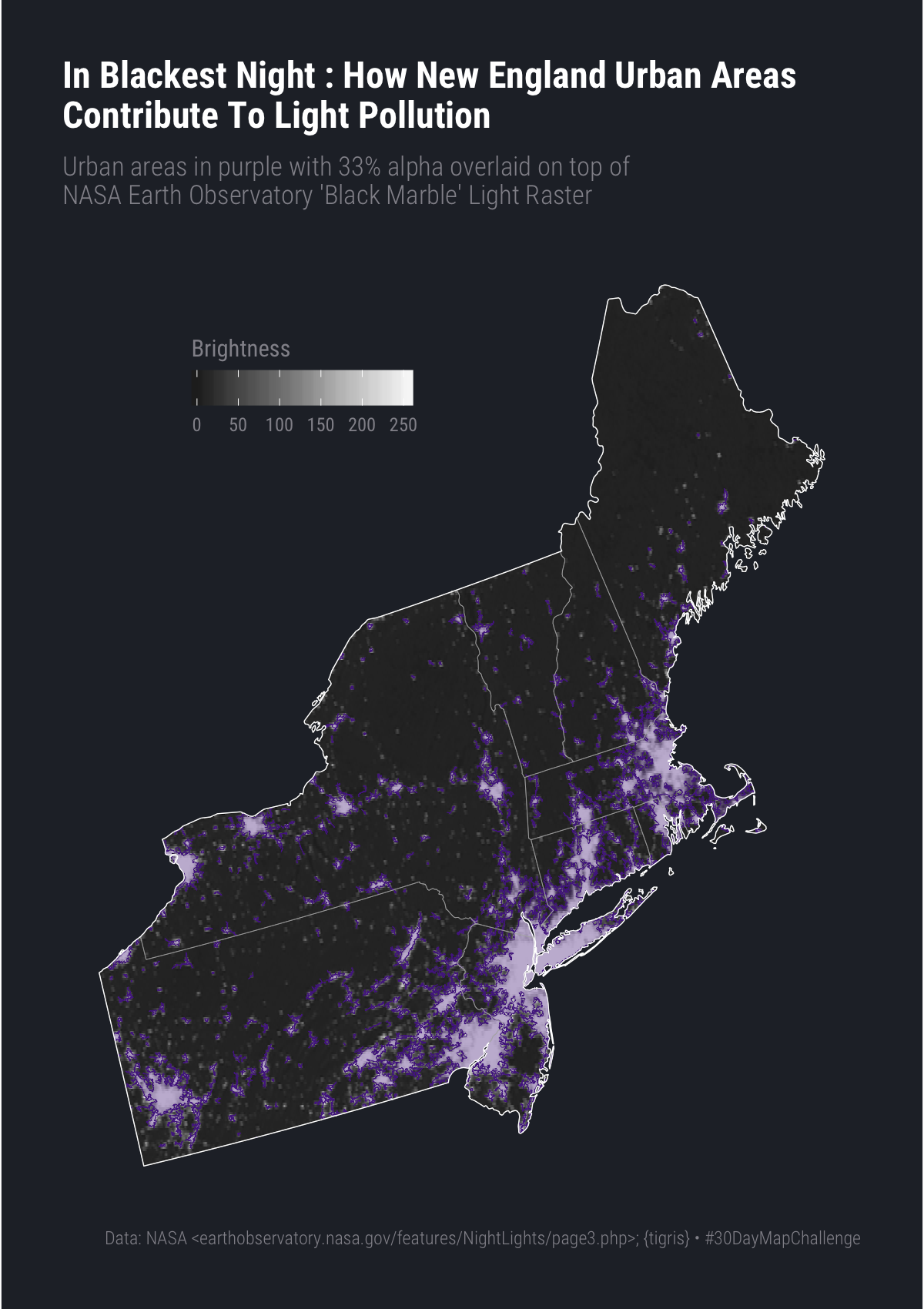
21.4 In Review
It’s Day 19 and you’re hopefully starting to see some idioms/patterns emerging when working with spatial data. Today, we introduced {raster} operations, which turn out to be much like {stars} operations (but {stars} is almost always faster and works better within the {sf} ecosystem).
21.5 Try This At Home
We noted that the Black Marble GeoTIFF was an older one. Grab a newer one and first perform the same operations, then “diff” the rasters and show what’s changed since 2016. You may want to use {stars} for this part.
Pick a different region of the world (if you use something outside the U.S. you’ll need to source other raster urban area data) and perform a similar set of operations.