17 Day 15: Names
17.1 Technologies/Techniques
- Scraping data with R for use in a map context
- Creating a silhouette of Maine for use in making a Maine shaped word cloud
- Prepping final data for use in another context
17.2 Data Source: Baby Names
The U.S. Social Security Administration maintains historical, popular baby names by state database that they’ve put online53. Where there may be a data file for this out there somewhere I just threw together a quick scraper for it vs spend time googling.
This is similar to what we’ve done in a previous challenge. We make a custom scraping function from a captured cURL request and then grab and cache the data.
if (!file.exists(here::here("data/maine-names.rds"))) {

  cURL <- "curl 'https://www.ssa.gov/cgi-bin/namesbystate.cgi' -H 'Connection: keep-alive' -H 'Cache-Control: max-age=0' -H 'DNT: 1' -H 'Upgrade-Insecure-Requests: 1' -H 'User-Agent: Mozilla/5.0 (Macintosh; Intel Mac OS X 10_15_2) AppleWebKit/537.36 (KHTML, like Gecko) Chrome/79.0.3945.36 Safari/537.36' -H 'Sec-Fetch-User: ?1' -H 'Origin: https://www.ssa.gov' -H 'Content-Type: application/x-www-form-urlencoded' -H 'Accept: text/html,application/xhtml+xml,application/xml;q=0.9,image/webp,image/apng,*/*;q=0.8,application/signed-exchange;v=b3;q=0.9' -H 'Sec-Fetch-Site: same-origin' -H 'Sec-Fetch-Mode: navigate' -H 'Referer: https://www.ssa.gov/cgi-bin/namesbystate.cgi' -H 'Accept-Encoding: gzip, deflate, br' -H 'Accept-Language: en-US,en;q=0.9,la;q=0.8' -H 'Cookie: TS014661b0=01cfd667a591a309251d155252645f7ba8d3e92ca313a0cc50797331d66b9eca4cda5b1bf09262fc2dd204124dd994ed097d2b0147; TS01838516=017e2f91c304e1561be5e212ee69533011530d7386dacfbaf9306ecd64d33947273a6a054c612f05721de9c9378d41fde9c08cf713' --data 'state=ME&year=2017' --compressed"

  straighten() %>%
    make_req() -> req

  get_names <- function(yr = 2018) {

    httr::POST(
      url = "https://www.ssa.gov/cgi-bin/namesbystate.cgi",
      body = list(
        state = "ME",
        year = as.character(yr)
      ),
      encode = "form"
    ) -> res

    out <- httr::content(res, as = "parsed", encoding = "UTF-8")

    html_node(out, xpath = ".//table[@bordercolor = '#aaabbb']") %>%
      html_table(header = TRUE, trim = TRUE) %>%
      as_tibble() %>%
      janitor::clean_names() %>%
      mutate(year = yr)

  }

  maine_names <- map_df(1960:2018, get_names)

  saveRDS(maine_names, here::here("data/maine-names.rds"))

}

maine_names <- readRDS(here::here("data/maine-names.rds"))

glimpse(maine_names)
## Observations: 5,900
## Variables: 6
## $ rank              <int> 1, 2, 3, 4, 5, 6, 7, 8, 9, 10, 11, 12, 13, 14, 15, …
## $ male_name         <chr> "David", "Michael", "Robert", "James", "John", "Mar…
## $ number_of_males   <int> 590, 582, 405, 390, 378, 362, 344, 243, 235, 212, 2…
## $ female_name       <chr> "Susan", "Linda", "Brenda", "Karen", "Donna", "Lisa…
## $ number_of_females <int> 280, 227, 224, 221, 220, 218, 210, 205, 166, 163, 1…
## $ year              <int> 1960, 1960, 1960, 1960, 1960, 1960, 1960, 1960, 196…
17.3 Prepping Our Word Cloud Map and Data
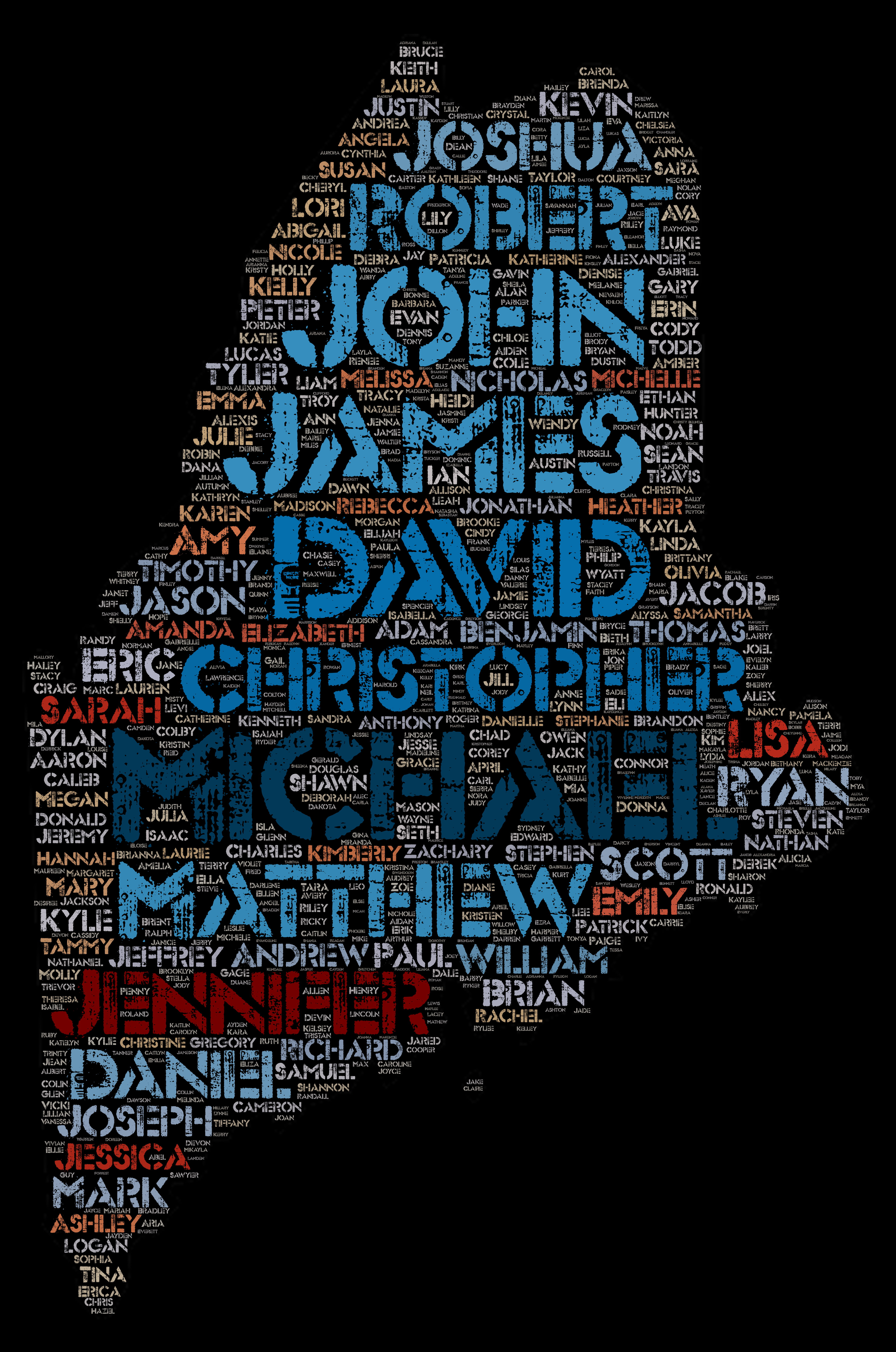
We’re going to kinda cheat and use WordArt.com54 for our final product since they have a nicer word cloud generator than anything available in R or Python (I include the latter since we can easily use icky Python from R when necessary).
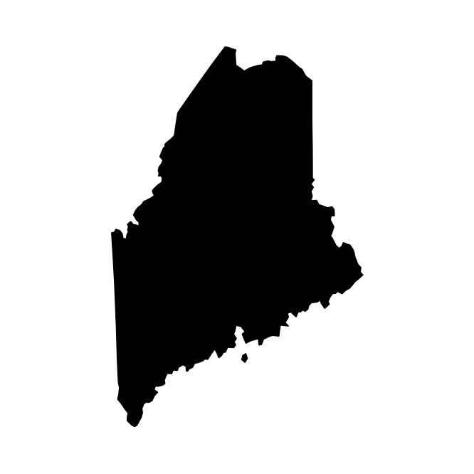
We’re going to use one of the more interesting features of WordArt.com and have the word cloud take the shape of an input silhouette image. In our case, this is Maine. We’re just making a solid black Maine image and writing it out:
if (!file.exists(here::here("img/me-silhouette.png"))) {

  st_read(here::here("data/me-counties.json")) %>%
    st_set_crs(4326) -> maine

  ggplot() +
    geom_sf(data = maine, fill = "black", color = "black") +
    coord_sf(datum = NA) +
    theme_ipsum_es(grid="") +
    theme(axis.text = element_blank()) -> gg

  ggsave(here::here("img/me-silhouette.png"), plot = gg, width = 500/72, height = 500/72, dpi = 96)

}
The WordArt.com site lets us specify colors as well as frequency so we can use two different palettes for SSA categories and compute the color based on the in-year frequency:
maine_names %>%
  {
    bind_rows(
      select(., name = male_name, ct = number_of_males) %>%
        count(name, wt = ct, name = "ct") %>%
        mutate(color = scales::brewer_pal(palette = "PuBu")(9)[cut(ct, 9)]),
      select(., name = female_name, ct = number_of_females) %>%
        count(name, wt = ct, name = "ct") %>%
        mutate(color = scales::brewer_pal(palette="OrRd")(9)[cut(ct, 9)])
    ) %>%
      arrange(desc(ct))
  } %>%
  write_delim(here::here("data/wordart.csv"), delim=";", col_names = FALSE) -> wc_df

glimpse(wc_df)
## Observations: 780
## Variables: 3
## $ name  <chr> "Michael", "Christopher", "David", "James", "Matthew", "John", …
## $ ct    <int> 13421, 9232, 9140, 8306, 8205, 7927, 7520, 6879, 6399, 6205, 60…
## $ color <chr> "#023858", "#0570B0", "#0570B0", "#3690C0", "#3690C0", "#3690C0…
17.4 Drawing the Map
This is really “upload the PNG and CSV to WordArt.com and play with remaining aesthetics”. It’s great fun!
17.5 In Review
We used R for data gathering, data prep, and making a silhouette for use in other programs. While I try to do as much as I can in R, sometimes you need to go outside of R to get things just the way you’re looking for.
17.6 Try This At Home
Try this with your state data!
There are a couple word cloud packages for R that can get close to this finished product. Give them a go and see if the effort to get to a similar end-results justifies the time spent.