18 Day 16: Places

18.1 Technologies/Techniques

Taking inspiration from Day 1 ({sf}, {ggplot2}, geom_sf())
Web scraping
More use of {rgeocodio}

18.2 Data Source: The Retail Apocalypse

I track a few different happenings in the world, one of which is the “retail apocalypse”⁵⁵. I’ve been collecting this data for a bit, but we’ll use some scraping techniques to pull lists from Business Insider, too.

My first thought for “places” was “places impacted by something” and losing these resources and jobs is pretty tough on a region despite the “great” economy we’re supposed to be in.

library(sf)
library(rvest)
library(ggthemes)
library(stringi)
library(pdftools)
library(hrbrthemes)
library(rgeocodio)
library(albersusa)
library(magrittr)
library(tidyverse)

We’ll do the scraping first, along with some more

if (!file.exists(here::here("data/russe.rds"))) {
  russe_pg <- read_html("https://www.businessinsider.com/charlotte-russe-bankruptcy-stores-closing-list-2019-2")

  # the lists are actually in ul/li lists!
  
  html_nodes(russe_pg, xpath=".//p[contains(., 'of the closing')]/following-sibling::ul/li") %>%
    html_text() -> russe

  russe_g <- rgeocodio::gio_batch_geocode(russe)

  saveRDS(russe_g, here::here("data/russe.rds"))
  
}

russe_g <- readRDS(here::here("data/russe.rds"))

if (!file.exists(here::here("data/sears.rds"))) {
  
  # the lists are actually in ul/li lists here too!
  
  # but we need to do some XPath surgery to get them

  sears_pg <- read_html("https://www.businessinsider.com/sears-closes-80-more-stores-2018-12")
  html_nodes(sears_pg, xpath=".//span[contains(., 'of the latest')]/../../p") %>%
    html_text() %>%
    keep(stri_detect_regex, "^(Sears|Kmart)") %>%
    stri_replace_first_regex("^(Sears[\\*]*|Kmart)", "") %>%
    stri_trim_both() -> sears

  sears2_pg <- read_html("https://www.businessinsider.com/sears-kmart-stores-closing-list-2018-10")
  html_nodes(sears2_pg, xpath=".//h2[text()='Sears' or text()='Kmart']/following-sibling::ul/li ") %>%
    html_text() %>%
    stri_trim_both() -> sears2

  sears_g <- rgeocodio::gio_batch_geocode(c(sears, sears2))
  
  saveRDS(sears_g, here::here("data/sears.rds"))

}

sears_g <- readRDS(here::here("data/sears.rds"))

# some previously scraped/geolocated data

if (!all(file.exists(here::here("data", c("dressbarn.rds", "payless.rds"))))) {

  dressbarn <- as_tibble(jsonlite::stream_in(gzcon(url("https://rud.is/dl/dressbarn-locations.json.gz"))))
  
  payless <- read_csv("http://rud.is/dl/2019-payless-store-closings.csv")
  
  saveRDS(dressbarn, here::here("data/dressbarn.rds"))
  saveRDS(payless, here::here("data/payless.rds"))
  
}

dressbarn <- readRDS(here::here("data/dressbarn.rds"))
payless <- readRDS(here::here("data/payless.rds"))

Let’s smush them all together with some useful labels:

bind_rows(
  filter(sears_g, map_lgl(response_results, ~nrow(.x) > 0)) %>% # find all valid geolocated data
    mutate(ll = map(response_results, ~select(.x, location.lng, location.lat) %>% slice(1))) %>% # pick the first geolocation result
    select(ll) %>%
    unnest(ll) %>%
    set_names(c("lng", "lat")) %>%
    mutate(brand = "Sears/Kmart"),

# lather, rinse, repeat  

  filter(russe_g, map_lgl(response_results, ~nrow(.x) > 0)) %>%
    mutate(ll = map(response_results, ~select(.x, location.lng, location.lat) %>% slice(1))) %>%
    select(ll) %>%
    unnest(ll) %>%
    set_names(c("lng", "lat")) %>%
    mutate(brand = "Russe"),

  select(payless, lng = longitude, lat=latitude) %>%
    mutate(brand = "Payless"),

  select(dressbarn, lng = lon, lat) %>%
    mutate(brand = "Dressbarn")
) %>%
  filter(lng > -130, lat > 21) -> continental # only looking for the conterminus U.S. 

glimpse(continental)
## Observations: 3,091
## Variables: 3
## $ lng   <dbl> -71.47046, -110.84236, -121.24129, -117.21061, -118.31655, -120…
## $ lat   <dbl> 42.07650, 32.22220, 37.93758, 34.47053, 34.18766, 34.90751, 38.…
## $ brand <chr> "Sears/Kmart", "Sears/Kmart", "Sears/Kmart", "Sears/Kmart", "Se…

Now, we’ll turn our plain ol’ data frame into an {sf} object:

# Load up Albers composite USA at the same time, but just the conterminus U.S. 
usa <- usa_sf("laea") %>% filter(!(name %in% c("Alaska", "Hawaii")))

# make a spatial version of the data frame
st_as_sf(continental, coords = c("lng", "lat"), crs = us_longlat_proj) %>%
  st_transform(albersusa::us_laea_proj) -> continental

glimpse(continental)
## Observations: 3,091
## Variables: 2
## $ brand    <chr> "Sears/Kmart", "Sears/Kmart", "Sears/Kmart", "Sears/Kmart", …
## $ geometry <POINT [m]> POINT (2296208 82451.33), POINT (-1022963 -1353086), P…

18.3 Drawing the Map

Now, we’ll draw points, mapping brands to a color aesthetic to see what kinds of damage was done and which company was involved:

ggplot() +
  geom_sf(data = usa, fill = "#252525", size = 0.125, color = "#b2b2b277") +
  geom_sf(data = continental, aes(color = brand), size = 0.25, alpha = 1/3, show.legend = "point") +
  scale_color_tableau(name = NULL) +
  coord_sf(datum = NA) +
  guides(
    colour = guide_legend(
      override.aes = list(size = 2, alpha=1)
    )
  ) +
  labs(
    x = NULL, y = NULL,
    title = "Places of the 2019 Retail Apocalpyse",
    subtitle = "Locations of four major brands store closings in 2019 alone (~3,100 stores in total)",
    caption = "Data source: (various + {rgeocodio}) • #30DayMapChallenge"
  ) +
  theme_ft_rc(grid="") +
  theme(legend.position = c(0.5, 0.95)) +
  theme(legend.direction = "horizontal") +
  theme(axis.text = element_blank())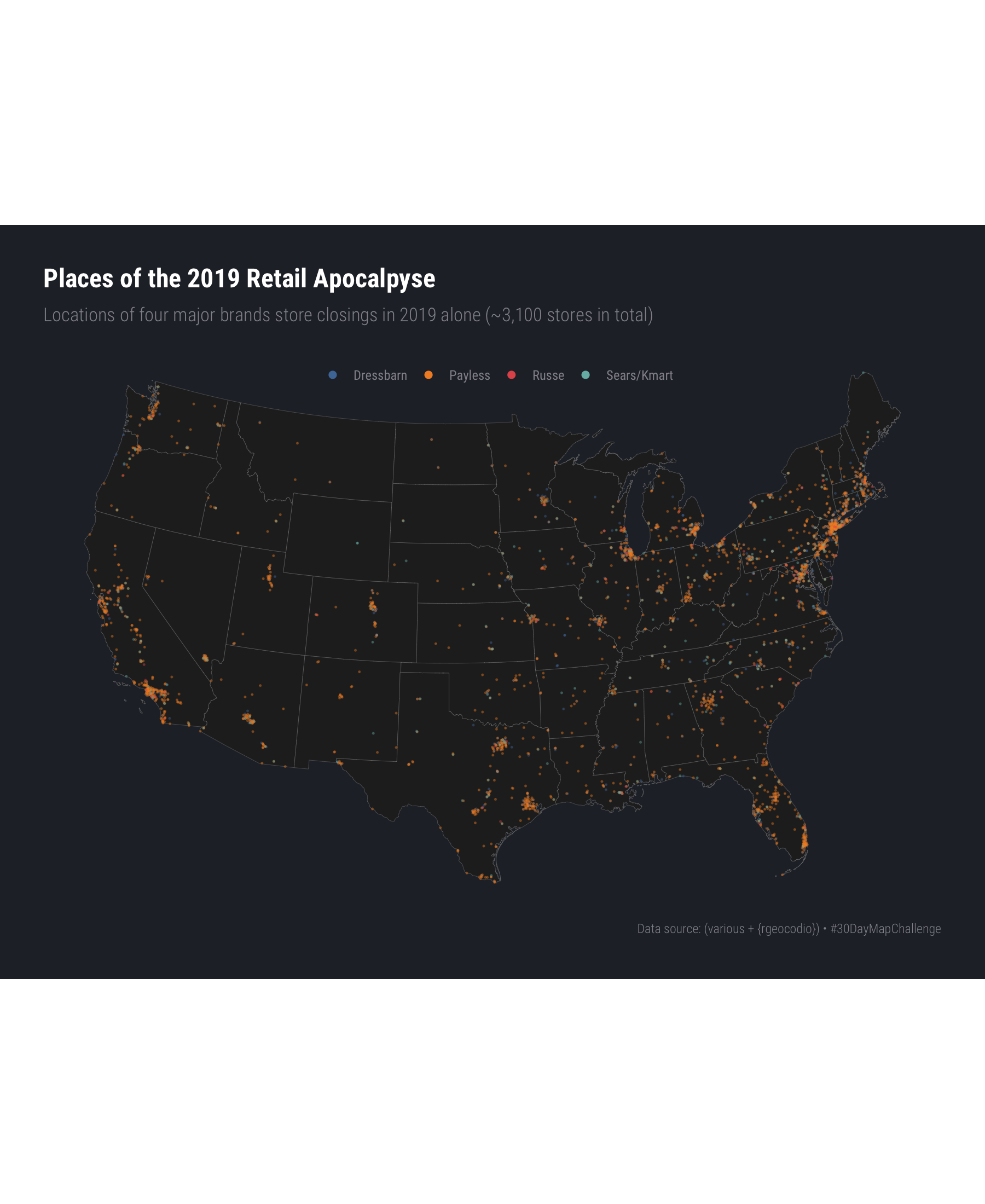

18.4 In Review

We told a short story with today’s challenge by showing the places across the U.S. that have been impacted in some way by the “retail apocalypse”. We also mapped aesthetics to points vs use facets.

18.5 Try This At Home

Dig into the data a bit and try to compute actual job and tax revenue impact and plot that on a different version fo the map.

Bin the data (perhaps using the hexbin technique from a previous challenge) and show impact by those bins.

https://en.wikipedia.org/wiki/Retail_apocalypse ↩︎