23 Day 21: Environment

23.1 Technologies/Techniques

Using external TopoJSON data
Working with {tigris}
“Zooming” in with map panels via {patchwork}
Using {sf} / geom_sf()

23.2 Data Source: Sea Rise Impact Forecast

Global warming is “a thing” and sea-level rise has been a phenomenon that many coastal communities have had to deal with for quite some time now. I wanted to see how sea-level rise would impact my environment. Thankfully, NASA makes that easy with their Sea Level Rise Datasets⁶² which are predictions based off on historical observations sound science.

library(sf)
library(tigris)
library(patchwork)
library(hrbrthemes)
library(tidyverse)

We’re going to incorporate a few shapefiles for this exercise. First, we’ll use the Maine county file we’ve been using in a number of the challenges, then grab a set of Maine town data to help annotate our maps. Since we’re going to create “zoom” panels, we’ll also extract York county (where I live) from the Maine country {sf} object.

st_read(here::here("data/me-counties.json")) %>%
  st_set_crs(4326) %>%
  st_transform("+proj=longlat +ellps=GRS80 +towgs84=0,0,0,0,0,0,0 +no_defs") -> maine
## Reading layer `cb_2015_maine_county_20m' from data source `/Users/hrbrmstr/books/30-day-map-challenge/data/me-counties.json' using driver `TopoJSON'
## Simple feature collection with 16 features and 10 fields
## geometry type:  MULTIPOLYGON
## dimension:      XY
## bbox:           xmin: -71.08434 ymin: 43.05975 xmax: -66.9502 ymax: 47.45684
## epsg (SRID):    NA
## proj4string:    NA

if (!file.exists(here::here("data/me-topo.geojson"))) {
  download.file("http://techslides.com/demos/d3/us/data/me.topo.json", here::here("data/me-topo.geojson"))
}

st_read(here::here("data/me-topo.geojson")) %>%
  st_set_crs(4326) %>%
  st_transform("+proj=longlat +ellps=GRS80 +towgs84=0,0,0,0,0,0,0 +no_defs") -> towns
## Reading layer `me' from data source `/Users/hrbrmstr/books/30-day-map-challenge/data/me-topo.geojson' using driver `TopoJSON'
## Simple feature collection with 985 features and 1 field
## geometry type:  POLYGON
## dimension:      XY
## bbox:           xmin: -71.08015 ymin: 43.06516 xmax: -66.95141 ymax: 47.4599
## epsg (SRID):    NA
## proj4string:    NA

filter(maine, NAME == "York") -> york

We’ll increase the annotation level with rivers and area water polygons from {tigris} then download the sea-level rise data set for Maine:

rivers <- linear_water(state = "ME", "York", class="sf")
water <- area_water(state = "ME", "York", class = "sf")

if (!file.exists(here::here("data/ME_West_slr_data_dist.zip"))) {
  
  download.file( 
    url = "https://coast.noaa.gov/htdata/Inundation/SLR/SLRdata/NewEngland/ME_West_slr_data_dist.zip",
    destfile = here::here("data/ME_West_slr_data_dist.zip")
  )
  
  unzip(
    zipfile = here::here("data/ME_West_slr_data_dist.zip"),
    exdir = here::here("data/ME_West_slr_data_dist")
  )
  
}

The NASA data is geodatabase⁶³ which is just another way to store/organize spatial data. They have many benefits over “shapefiles” including speed. We’ll take a look at the spatial data layers available to us. You can read more about geodatabases over at GIS Geography⁶⁴.

dsn <- here::here("data/ME_West_slr_data_dist/ME_West_slr_final_dist.gdb/")

st_layers(dsn)
## Driver: OpenFileGDB 
## Available layers:
##          layer_name geometry_type features fields
## 1   ME_West_low_0ft Multi Polygon      234      4
## 2  ME_West_low_10ft Multi Polygon      316      4
## 3   ME_West_low_1ft Multi Polygon      339      4
## 4   ME_West_low_2ft Multi Polygon      323      4
## 5   ME_West_low_3ft Multi Polygon      466      4
## 6   ME_West_low_4ft Multi Polygon      583      4
## 7   ME_West_low_5ft Multi Polygon      563      4
## 8   ME_West_low_6ft Multi Polygon      495      4
## 9   ME_West_low_7ft Multi Polygon      380      4
## 10  ME_West_low_8ft Multi Polygon      325      4
## 11  ME_West_low_9ft Multi Polygon      313      4
## 12  ME_West_slr_0ft Multi Polygon     1039      4
## 13 ME_West_slr_10ft Multi Polygon      956      4
## 14  ME_West_slr_1ft Multi Polygon     1067      4
## 15  ME_West_slr_2ft Multi Polygon      570      4
## 16  ME_West_slr_3ft Multi Polygon      597      4
## 17  ME_West_slr_4ft Multi Polygon      564      4
## 18  ME_West_slr_5ft Multi Polygon      632      4
## 19  ME_West_slr_6ft Multi Polygon      710      4
## 20  ME_West_slr_7ft Multi Polygon      758      4
## 21  ME_West_slr_8ft Multi Polygon      879      4
## 22  ME_West_slr_9ft Multi Polygon      982      4

These layers are named fairly well, Let’s load up both the 1 foot and 10 foot data and limit our view to York county. There are quite a few polygons per layer, so this is going to take some time. We’re using the low layer (that appears to be “low lying areas”) as the slr layers have complex/large polygons and take forever to process (I’m working on thinning these out for an update at some point).

if (!all(file.exists(here::here("data", c("ft01.rds", "ft10.rds"))))) {
  
  ft01 <- st_read(dsn, "ME_West_low_1ft")
  ft01 <- st_intersection(st_buffer(ft01, 0), york)
  
  ft10 <- st_read(dsn, "ME_West_low_10ft")
  ft10 <- st_intersection(st_buffer(ft10, 0), york)
  
  saveRDS(ft01, here::here("data/ft01.rds"))
  saveRDS(ft10, here::here("data/ft10.rds"))
  
}

ft01 <- readRDS(here::here("data/ft01.rds"))
ft10 <- readRDS(here::here("data/ft10.rds"))

Finally, let’s also limit towns to just those in York county:

york_towns <- st_intersection(st_buffer(towns, 0), york)

23.3 Drawing the Map

We’re going to use {patchwork} to make three side-by-side panels that let us zoom in on the areas closer to me. We’ll color the sea level data in red and resort to using a third-party program to manually add in zoom lines as it was faster than trying to add those with some {grid} hacks or {magick} incantations.

ggplot() +
  geom_sf(data = maine, fill = "#efefef", size = 0.25) +
  geom_sf(data = york, fill = "#efefef", size = 0.125) +
  # geom_sf(data = water, fill = "#8cb6d3", color = "#8cb6d3") +
  geom_sf(data = rivers, size = 0.075, color = "#8cb6d366") +
  geom_sf(data = ft01, fill = "#bd002666", color = "#bd002666") +
  geom_sf_text(data = maine, aes(label = NAME), family = font_es_bold, size = 3.25, color="white") +
  geom_sf_text(data = maine, aes(label = NAME), family = font_es_light, size = 3) +
  coord_sf(datum = NA) +
  labs(
    x = NULL, y = NULL
  ) +
  theme_ipsum_es(grid="") -> gg

ggplot() +
  geom_sf(data = york, fill = "#efefef", size = 0.25) +
  geom_sf(data = water, fill = "#8cb6d3", color = "#8cb6d3") +
  geom_sf(data = rivers, size = 0.1, color = "#8cb6d3") +
  geom_sf_text(data = york_towns, aes(label = id), family = font_es_bold, size = 2.25, color="white") +
  geom_sf_text(data = york_towns, aes(label = id), family = font_es_light, size = 2) +
  geom_sf(data = ft01, fill = "#bd002666", color = "#bd002666") +
  coord_sf(datum = NA) +
  labs(
    x = NULL, y = NULL
  ) +
  theme_ipsum_es(grid="") -> gg1

ggplot() +
  geom_sf(data = york, fill = "#efefef", size = 0.25) +
  geom_sf(data = water, fill = "#8cb6d3", color = "#8cb6d3") +
  geom_sf(data = rivers, size = 0.1, color = "#8cb6d3") +
  geom_sf(data = ft01, fill = "#bd002666", color = "#bd002666") +
  geom_sf_text(data = york_towns, aes(label = id), family = font_es_bold, size = 4.25, color="white") +
  geom_sf_text(data = york_towns, aes(label = id), family = font_es_light, size = 4) +
  coord_sf(datum = NA, xlim=c(-70.84655, -70.577334), ylim=c(43.061743, 43.216308)) +
  labs(
    x = NULL, y = NULL
  ) +
  theme_ipsum_es(grid="") -> gg2

gg + gg1 + gg2 + plot_layout(ncol = 3)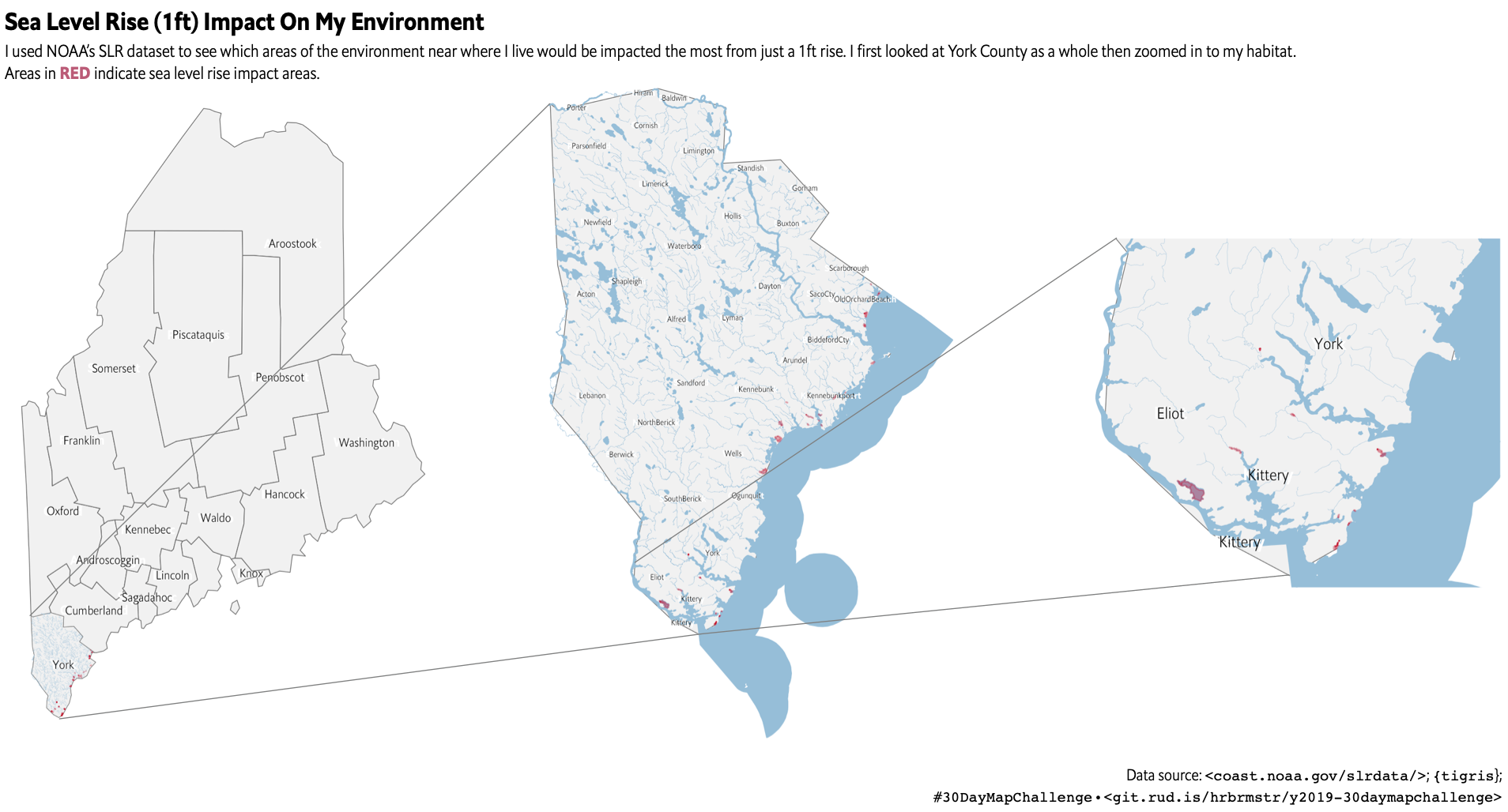

23.4 In Review

We used a new spatial file type and incorporated layers from many sources to create a composite panel-zoom view of sea-level rise in my neck of the woods.

23.5 Try This At Home

Do this for your area!

Work on using the slr layers for your area and potentially generate more usable data sources for the R spatial community before I get a chunk of time to do the same thing.