Data Source: The Divine Comedy
library(sf)
library(igraph)
library(ggraph)
library(ggtext)
library(hrbrthemes)
library(tidyverse)
world <- rnaturalearth::ne_countries(returnclass = "sf")

if (!file.exists(here::here("data/dante.json"))) {
  download.file(
    url = "https://www.mappingdante.com/network/data.json",
    destfile = here::here("data/dante.json")
  )
}

dante <- jsonlite::fromJSON(here::here("data/dante.json"))

graph_from_data_frame(
  select(dante$edges, source, target, col = color) %>%
    mutate(col = map_chr(col, ~{
      gsub("[^[:digit:]]", " ", .x) %>%
        trimws() %>%
        strsplit(" ", fixed=TRUE) %>%
        unlist() %>%
        as.integer() %>%
        `/`(255) -> x
      rgb(x[1], x[2], x[3])
    })),
  vertices = select(dante$nodes, id, label, col=color, size) %>%
    mutate(col = map_chr(col, ~{
      gsub("[^[:digit:]]", " ", .x) %>%
        trimws() %>%
        strsplit(" ", fixed=TRUE) %>%
        unlist() %>%
        as.integer() %>%
        `/`(255) -> x
      rgb(x[1], x[2], x[3])
    })) %>%
    mutate(lab = ifelse(size >= 60, sprintf("%s    ", label), ""))
) -> g

select(dante$nodes, x, y) %>%
  as.matrix() -> l
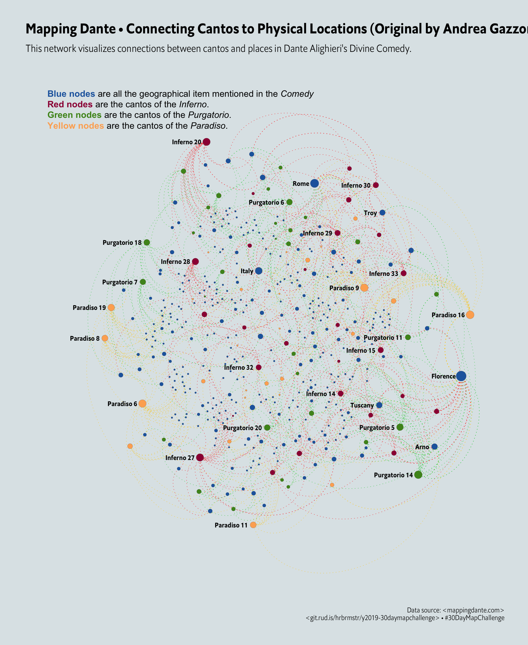
Drawing the Map
ggraph(g, layout = l) +
  geom_edge_arc2(
    aes(color = I(col)), width = 0.25, linetype = "dotted", alpha=2/3
  ) +
  geom_node_point(
    aes(size = size, fill = I(col)),
    shape = 21, color = "#2b2b2b", stroke = 0.075
  ) +
  geom_node_text(
    aes(label = lab), hjust = 1, family = font_es_bold, size = 3
  ) +
  geom_richtext(
    data = data.frame(),
    aes(
      x = -2900,
      y = -2900,
      label = paste0(c(
        "<span style='color:#2166ac'>**Blue nodes**</span> are all the geographical item mentioned in the *Comedy*",
        "<span style='color:#9d1642'>**Red nodes**</span> are the cantos of the *Inferno*.",
        "<span style='color:#4d9220'>**Green nodes**</span> are the cantos of the *Purgatorio*.",
        "<span style='color:#fdae61'>**Yellow nodes**</span> are the cantos of the *Paradiso*."
      ), collapse = "<br/>\n")
    ),
    hjust = 0, size = 4, vjust = 1,
    fill = NA, label.color = NA,
    label.padding = grid::unit(rep(0, 4), "pt")
  ) +
  scale_y_reverse() +
  scale_fill_manual(
    name = "",
    values = c(
      "#00CC00" = "#4d9221",
      "#00CC33" = "#00cc33",
      "#FF0000" = "#9e0142",
      "#FF3333" = "#ff3333",
      "#0000FF" = "#2166ac",
      "#FFCC00" = "#fdae61"
    ),
    label = c(
      "#FFCC00" = "Paradiso",
      "#FF0000" = "Inferno",
      "#00CC00" = "Purgatorio"#,
      # "#FF3333" = "#ff3333",
      # "#00CC33" = "#00cc33"
    ),
    breaks = c(
      "#FFCC00" = "Paradiso",
      "#FF0000" = "Inferno",
      "#00CC00" = "Purgatorio"
    )
  ) +
  guides(
    size = FALSE
  ) +
  labs(
    x = NULL, y = NULL,
    title = "Mapping Dante • Connecting Cantos to Physical Locations (Original by Andrea Gazzoni)",
    subtitle = "This network visualizes connections between cantos and places in Dante Alighieri's Divine Comedy.",
    caption = "Data source: <mappingdante.com>\n<git.rud.is/hrbrmstr/y2019-30daymapchallenge> • #30DayMapChallenge"
  ) +
  theme_ipsum_es(grid="") +
  theme(plot.background = element_rect(color = "#DEE5E8", fill = "#DEE5E8")) +
  theme(panel.background = element_rect(color = "#DEE5E8", fill = "#DEE5E8")) +
  theme(axis.text = element_blank())
as_tibble(dante$edges) %>%
pull(attributes) %>%
select(lng = Long_X, lat = Lat_Y) %>%
mutate_all(as.numeric) %>%
filter(complete.cases(.)) %>%
count(lng, lat) %>%
st_as_sf(coords = c("lng", "lat")) %>%
st_set_crs(st_crs(world)) -> all_places
st_intersection(all_places, select(world, name)) %>%
count(name, wt = n) %>%
filter(n <= 3) %>%
filter(!(name %in% c("Cyprus", "N. Cyprus"))) -> single_places
ggplot() +
geom_sf(
data = world, size = 0.125, linetype = "dotted",
fill = "#3B454A", color = "#b2b2b2"
) +
geom_sf(
data = all_places,
aes(size = n), shape=21, stroke = 0.125,
fill = alpha("#fdae61", 2/3), color = "white", show.legend = FALSE
) +
geom_sf_label(
data = single_places,
aes(
label = name,
hjust = I(ifelse(name %in% c("Morocco", "Switzerland", "Tunisia"), 1, 0))
),
color = "white", family = font_es_bold, size = 3,
vjust = 1, label.size = 0, fill = alpha("black", 1/10)
) +
coord_sf(
xlim = c(-10, 80),
ylim = c(-1, 75),
datum = NA
) +
labs(
x = NULL, y = NULL,
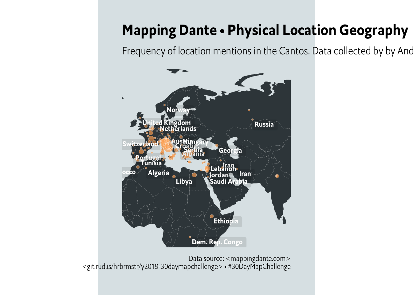
title = "Mapping Dante • Physical Location Geography",
subtitle = "Frequency of location mentions in the Cantos. Data collected by by Andrea Gazzoni.",
caption = "Data source: <mappingdante.com>\n<git.rud.is/hrbrmstr/y2019-30daymapchallenge> • #30DayMapChallenge"
) +
theme_ipsum_es(grid="") +
theme(plot.background = element_rect(color = "#DEE5E8", fill = "#DEE5E8")) +
theme(panel.background = element_rect(color = "#DEE5E8", fill = "#DEE5E8")) +
theme(axis.text = element_blank())
st_intersection(all_places, select(world, name)) %>%
  count(name, wt = n) %>%
  # filter(n <= 10) %>%
  filter(!(name %in% c("Cyprus", "N. Cyprus"))) -> single_places

ggplot() +
  geom_sf(
    data = world, size = 0.125, linetype = "dotted",
    fill = "#3B454A", color = "#b2b2b2"
  ) +
  geom_sf(
    data = all_places,
    aes(size = n), shape=21, stroke = 0.125,
    fill = alpha("#fdae61", 2/3), color = "white", show.legend = FALSE
  ) +
  geom_sf_label(
    data = single_places,
    aes(
      label = name,
      hjust = I(ifelse(name %in% c("Morocco", "Switzerland", "Tunisia"), 1, 0))
    ),
    color = "white", family = font_es_bold, size = 3,
    vjust = 1, label.size = 0, fill = alpha("black", 1/10)
  ) +
  coord_sf(
    xlim = c(0, 30),
    ylim = c(35, 50),
    datum = NA
  ) +
  labs(
    x = NULL, y = NULL,
    title = "Mapping Dante • Physical Location Geography • Italy Zoom",
    subtitle = "Frequency of location mentions in the Cantos. Data collected by by Andrea Gazzoni.",
    caption = "Data source: <mappingdante.com>\n<git.rud.is/hrbrmstr/y2019-30daymapchallenge> • #30DayMapChallenge"
  ) +
  theme_ipsum_es(grid="") +
  theme(plot.background = element_rect(color = "#DEE5E8", fill = "#DEE5E8")) +
  theme(panel.background = element_rect(color = "#DEE5E8", fill = "#DEE5E8")) +
  theme(axis.text = element_blank())
