5 Day 3: Polygons

5.1 Technologies/Techniques

Using a custom GeoJSON file with {sf}
Instrumenting a hidden API with {httr}
Using {ggplot2} geom_sf() to draw a map and stat_density_2d() to draw polygons on it

5.2 Data Source: Comcast XFINITY Hotspots

Most maps use polygons to draw features (i.e. each state on a U.S. map is most likely a polygon if the map isn’t a raster image) so today’s challenge could simply have been to just “draw a map”. I decided to do a bit more work than that and thought that making a polygon-based heatmap (a.k.a. filled 2D kernel density polygons) would make for an interesting entry.

Comcast — a U.S. internet provider — has a “hotspot locator” app²⁷ that customers can use to, well, locate Wi-Fi hotspots when they’re out and about. Just zoom around or enter a zip code to see a listing of all the hotspots in a given area.

The app makes an XHR request²⁸ for each search that looks a bit like this:

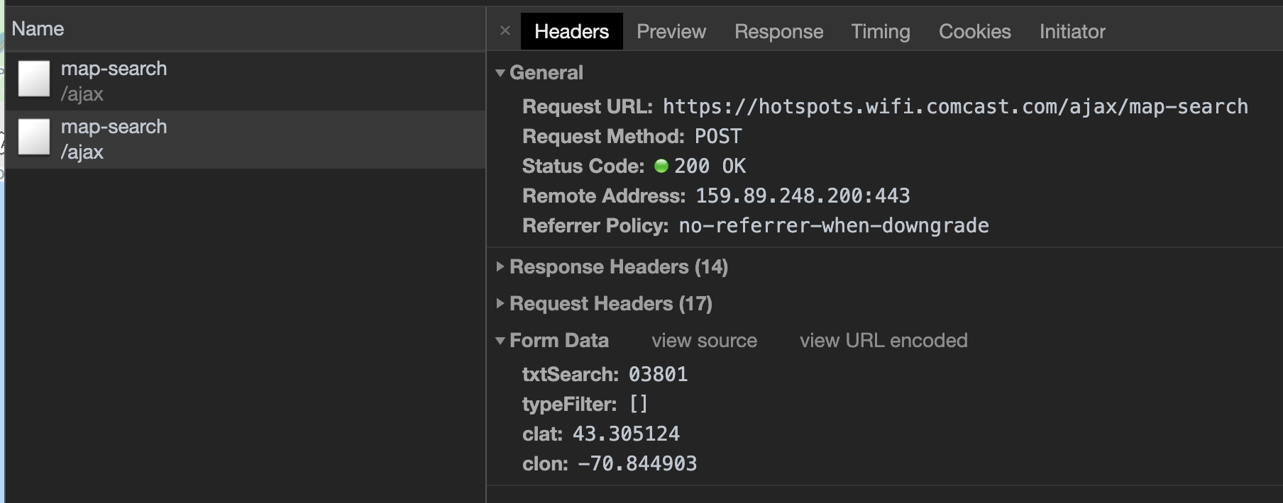
You can see the zipcode in the txtSearch parameter at the bottom.

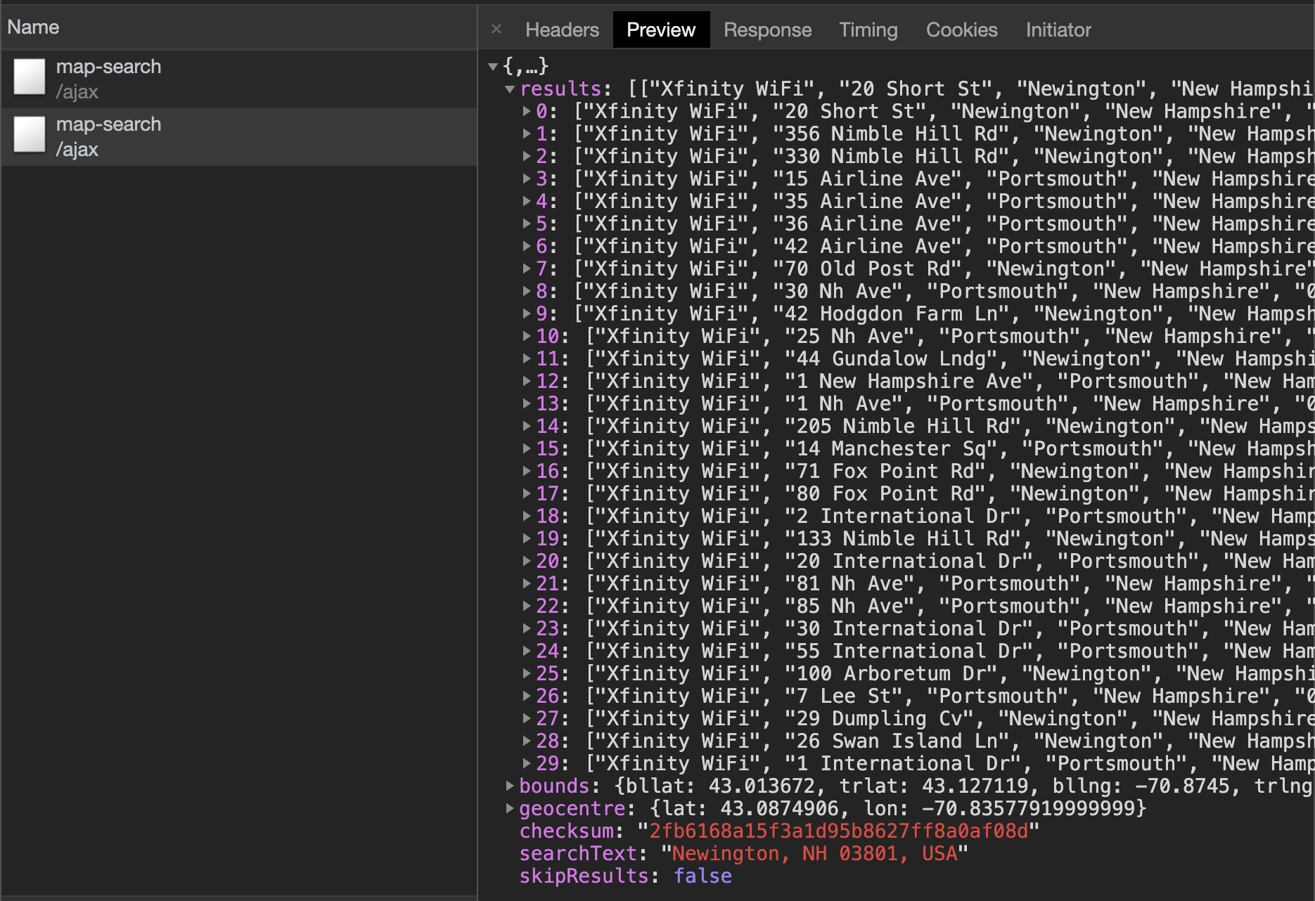
and returns a JSON result that looks like this:

5.3 Creating a Hidden API Scraper

We can use this hidden API to collect all the hotspots for a given set of zipcodes and then use those points to build a set of 2D kernel density polygons focusing on Maine.

I didn’t know if making a “bare” HTTP POST request would work since these apps sometimes look for special headers that help “prove” you’re using a browser and not a scraper, so I used the “Copy as cURL” option on one of the map-search entries and passed it into {curlconverter}, which is a package that turns browser cURL request lines into a working R {httr} function:

library(sf)
library(glue)
library(curlconverter)
library(zipcode)
library(hrbrthemes)
library(tidyverse)

url <- "curl 'https://hotspots.wifi.comcast.com/ajax/map-search' -H 'Connection: keep-alive' -H 'sec-ch-ua: \"Google Chrome 79\"' -H 'Accept: application/json, text/javascript, */*; q=0.01' -H 'Sec-Fetch-Dest: empty' -H 'User-Agent: Mozilla/5.0 (Macintosh; Intel Mac OS X 10_15_1) AppleWebKit/537.36 (KHTML, like Gecko) Chrome/79.0.3945.16 Safari/537.36' -H 'DNT: 1' -H 'Content-Type: application/x-www-form-urlencoded; charset=UTF-8' -H 'Origin: https://hotspots.wifi.xfinity.com' -H 'Sec-Fetch-Site: cross-site' -H 'Sec-Fetch-Mode: cors' -H 'Referer: https://hotspots.wifi.xfinity.com/mobile/' -H 'Accept-Encoding: gzip, deflate, br' -H 'Accept-Language: en-US,en;q=0.9,la;q=0.8' --data 'txtSearch=03901&typeFilter=[]&clat=44.686349&clon=-68.904427' --compressed"

straighten(url) %>%
  make_req() -> req

The req object is a working function (i.e. you can call req() and it’ll do what the original cURL request did), but that function’s source code is also shown in the R console and put on the clipboard.

I pasted it from the clipboard and modified it to add a parameter for the zipcode and give it a name plus do some post-processing of the JSON to get the data into a data frame:

fetch_hotspots <- function(zip) {

  message(zip)

  httr::POST(
    url = "https://hotspots.wifi.comcast.com/ajax/map-search",
    httr::add_headers(
      Connection = "keep-alive",
      `sec-ch-ua` = "Google Chrome 79",
      Accept = "application/json, text/javascript, */*; q=0.01",
      `Sec-Fetch-Dest` = "empty",
      `User-Agent` = "Mozilla/5.0 (Macintosh; Intel Mac OS X 10_15_1) AppleWebKit/537.36 (KHTML, like Gecko) Chrome/79.0.3945.16 Safari/537.36",
      DNT = "1", Origin = "https://hotspots.wifi.xfinity.com",
      `Sec-Fetch-Site` = "cross-site",
      `Sec-Fetch-Mode` = "cors",
      Referer = "https://hotspots.wifi.xfinity.com/mobile/",
      `Accept-Encoding` = "gzip, deflate, br",
      `Accept-Language` = "en-US,en;q=0.9,la;q=0.8"
    ),
    body = list(
      txtSearch = zip,
      typeFilter = "[]",
      clat = "44.686349",
      clon = "-68.904427"
    ),
    encode = "form"
  ) -> res

  stop_for_status(res)

  out <- content(res, as = "text", encoding = "UTF-8")
  out <- jsonlite::fromJSON(out)

  if (length(out$results) == 0) return(NULL)

  out <- as_tibble(out$results)
  out <- select(out, lng=V7, lat=V6)
  out <- mutate_all(out, as.numeric)

  out

}

Now we can call it with a zipcode like this:

str(fetch_hotspots("03801"), 1)
## Classes 'tbl_df', 'tbl' and 'data.frame':    30 obs. of  2 variables:
##  $ lng: num  -70.8 -70.8 -70.8 -70.8 -70.8 ...
##  $ lat: num  43.1 43.1 43.1 43.1 43.1 ...

To fetch all the Maine hotspots we can use the {zipcode} package and just iterate through all the Maine ones, caching them since this takes a bit of time to run:

if (!file.exists(here::here("data/me-xfin-hotspots.rds"))) {

  data(zipcode)
  
  as_tibble(zipcode) %>%
    filter(state == "ME") %>%
    pull(zip) %>%
    map_df(fetch_hotspots) -> maine_xfin_hotspots

  saveRDS(maine_xfin_hotspots, here::here("data/me-xfin-hotspots.rds"))

}

maine_xfin_hotspots <- readRDS(here::here("data/me-xfin-hotspots.rds"))

5.4 Drawing the Map

I just happen to have a set of Maine county polygons handy in a GeoJSON²⁹ file since I use it every year to track just how poorly Central Maine Power does their job (we have many power outages).

Let’s read in the GeoJSON and then ensure the hotspots we’ve found are within the Maine bounding box (lots of ways to do this, here’s one).

Note the st_set_crs(4326) line right after the st_read(). This GeoJSON file has no coordinate reference system (CRS) set³⁰, so we need to give it one. I happen to know it definitely is EPSG:4326. What does that secret code mean?

“EPSG” stands for “European Petroleum Survey Group”. Said group maintains and publishes a database of coordinate system information along with related documents on map projections and datums³¹. “4326” is the reference number for the “WGS 84” CRS, i.e. the “World Geodetic System 1984”. For the sake of simplicity, think of it as the most basic, X (“longitude”) / Y (“latitude”) reference system grid. Technically it is “projected” since it’s taking a 3D sphere and putting it on a 2D surface, but this “latlong” projection isn’t great when you need to do things like measure distances accurately.

st_read(here::here("data/me-counties.json")) %>%
  st_set_crs(4326) -> maine 
## Reading layer `cb_2015_maine_county_20m' from data source `/Users/hrbrmstr/books/30-day-map-challenge/data/me-counties.json' using driver `TopoJSON'
## Simple feature collection with 16 features and 10 fields
## geometry type:  MULTIPOLYGON
## dimension:      XY
## bbox:           xmin: -71.08434 ymin: 43.05975 xmax: -66.9502 ymax: 47.45684
## epsg (SRID):    NA
## proj4string:    NA

bbox <- st_bbox(maine)

maine_xfin_hotspots %>%
  filter(
    between(lat, bbox$ymin, bbox$ymax),
    between(lng, bbox$xmin, bbox$xmax),
  ) -> maine_xfin_hotspots

glimpse(maine_xfin_hotspots)
## Observations: 4,817
## Variables: 2
## $ lng <dbl> -70.84987, -70.85362, -70.85499, -70.82253, -70.84057, -70.84057,…
## $ lat <dbl> 43.27697, 43.27415, 43.27300, 43.28539, 43.26015, 43.26015, 43.27…

The rest is surprisingly straightforward! Draw the Maine polygons with geom_sf() and then add a stat_density_2d() layer with the points we’ve collected. One reason this works is that we’ve left the Maine polygons in the default “latlong” projection, so we don’t need to do any extra work projecting the polygon information.

I did a bit of trial and error for the n and h parameters to stat_density_2d() and also chose to plot the points underneath the polygons to cover any areas that weren’t dense enough to have polygons generated.

ggplot() +
  geom_sf(
    data = maine, color = "#b2b2b2", size = 0.125, fill = "#3B454A"
  ) +
  geom_point(
     data = maine_xfin_hotspots, aes(lng, lat),
     size = 0.125, alpha=1/2, color = "white"
  ) +
  stat_density_2d(
   data = maine_xfin_hotspots, geom = "polygon",
   aes(lng, lat, fill = stat(level)), n = 1000, h = c(0.2, 0.2)
  ) +
  scale_fill_viridis_c(option = "magma", direction = -1) +
  coord_sf(datum = NA) +
  labs(
    x = NULL, y = NULL,
    title = "Xfinity Hotspot Coverage in Maine",
    subtitle = glue("{scales::comma(nrow(maine_xfin_hotspots))} total Xfinity hotspots in Maine\nPolygons show areas of highest hotspot density\nDots show individual hotspots"),
    caption = "Data source: <hotspots.wifi.xfinity.com/mobile/> • #30DayMapChallenge"
  ) +
  theme_ft_rc(grid="") +
  theme(axis.text = element_blank()) +
  theme(legend.position = "none")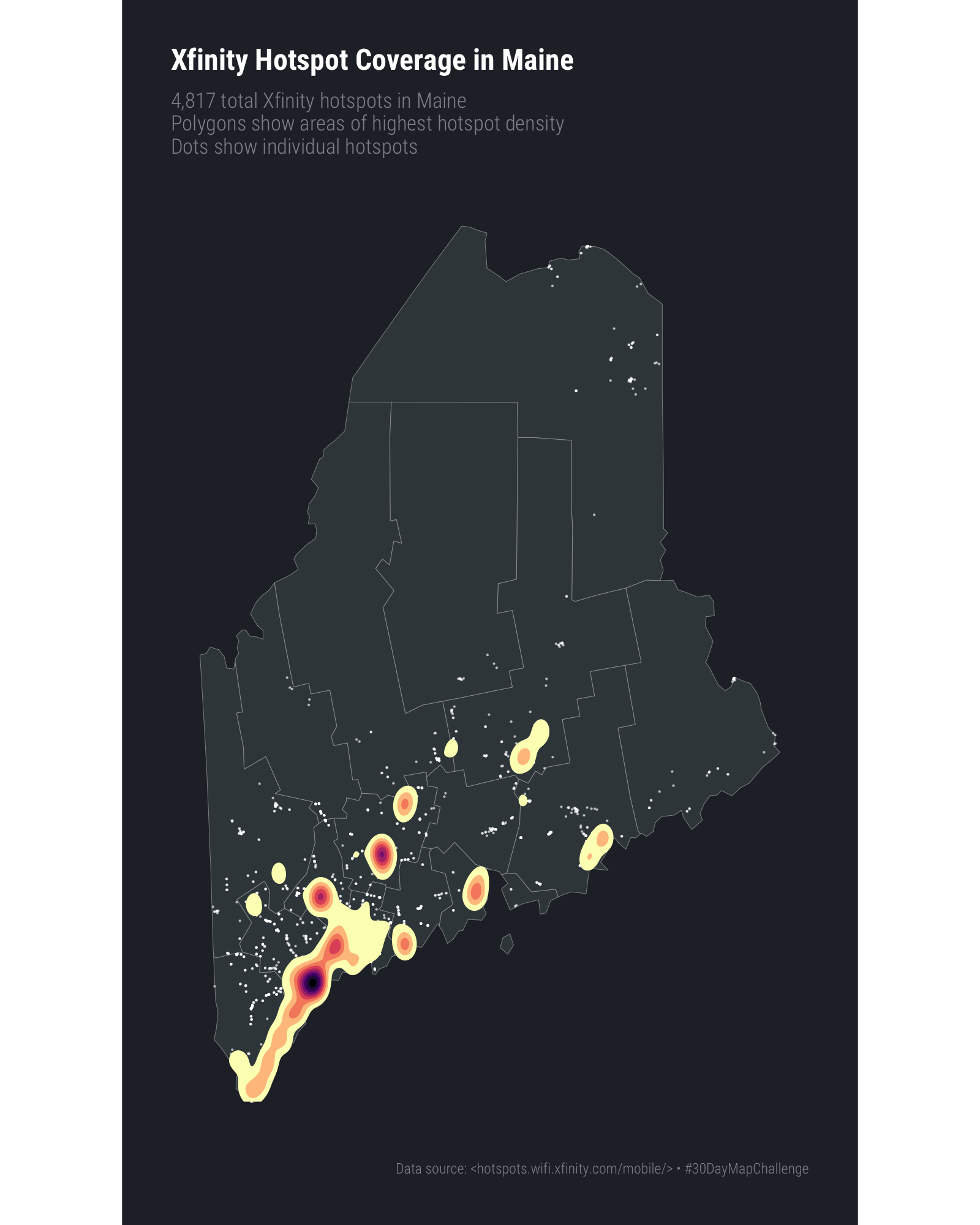

5.5 In Review

This exercise used the knowledge about mixing traditional and geom_sf() geoms from the previous challenge to build a new polygon layer and also used a new type of base map format (GeoJSON).

5.6 Try This At Home

Try passing in a different CRS to coord_sf() and see what happens (if anything) to the resultant map image.

Re-work the example to use a different state or multiple states as the base layer and gather up new points from the API. The NJ + NY + PA area has a super-high density of Comcast hotspots and should make for some interesting polygons.

https://hotspots.wifi.comcast.com/↩︎
https://www.w3schools.com/xml/xml_http.asp ↩︎
https://geojson.org/↩︎
Technically GeoJSON files default to this EPSG:4326 CRS↩︎
https://oceanservice.noaa.gov/facts/datum.html ↩︎