6 Day 4: Hex
6.1 Technologies/Techniques
- Using
{rnaturalearth}and separate ocean base layers - Building a hex grid in the
{sf}ecosystem - Binning incidents into hex grid locations
- Using
{ggplot2}geom_sf()to draw a map filled hex polygons
6.2 Data Source: Anti-Shipping Activity (PIRATES!)
I started maintaining a package ({asam}32) that lets folks work with “anti-shipping activity messages”33 maintained by the U.S. National Geospatial-Intelligence Agency when I began crafting my annual R-themed “Talk Like a Pirate Day” posts.
Each record in the ASAM database contains high level information on each incident, including longitude/latitude along with ship and offender metadata and a brief blurb on the incident. Most of these incidents are pirates and they’ve kept a log since 1978 of all these incidents. I thought a hex grid heatmap of all ASAM incidents since the database inception would be a fun way to meet today’s challenge.
I ended up having to tweak the {asam} package yet-again for this challenge since the maintainers changed the data source format.
6.3 Getting the Layers
We’re going to need two different map layers for this challenge. One is the old standby of ne_countries() from {rnaturalearth} so we can plot the countries/continents.
However, the ASAM database covers piracy on the water. To make a hexgrid heatmap of incidents, we’ll need an ocean layer to base it on and that doesn’t come with {rnaturalearth} so we’ll have to grab it ourselves34.
# get the world without antarctica
ne_countries(scale = "medium", returnclass = "sf") %>%
  filter(name != "Antarctica") %>%
  st_transform("+proj=eqearth +wktext") -> world

# get oceans
st_read(here::here("data/ocean/ne_110m_ocean.shp")) %>%
  select(scalerank, geometry) %>%
  st_transform("+proj=eqearth +wktext") -> ocean
## Reading layer `ne_110m_ocean' from data source `/Users/hrbrmstr/books/30-day-map-challenge/data/ocean/ne_110m_ocean.shp' using driver `ESRI Shapefile'
## Simple feature collection with 2 features and 2 fields
## geometry type:  POLYGON
## dimension:      XY
## bbox:           xmin: -180 ymin: -85.60904 xmax: 180 ymax: 90
## epsg (SRID):    4326
## proj4string:    +proj=longlat +datum=WGS84 +no_defs
6.4 Making the Grid
We need to convert the ocean layer to a grid and to do that we can use st_make_grid(). This process takes a bit so we’ll cache our work to speed up reproduction later on:
# make a grid from the oceans
if (!file.exists(here::here("data/ocean-grid-250.rds"))) {

  st_make_grid(
    ocean,
    n = c(250, 250), # grid granularity
    crs = st_crs(ocean),
    what = "polygons",
    square = FALSE # hex!
  ) -> grid

  grid <- st_sf(index = 1:length(lengths(grid)), grid)

  saveRDS(grid, here::here("data/ocean-grid-250.rds"))

}

grid <- readRDS(here::here("data/ocean-grid-250.rds"))
And, here’s the resultant grid:
ggplot() +
  geom_sf(data = grid, fill = "white", color = "black", size = 0.0725) +
  coord_sf(datum = NA) +
  theme_minimal()
6.5 Getting Pirate Data
The read_asam() function lets us grab the ASAM database but the server is pretty slow, so we’ll cache this result, too:
# get PIRATES!
if (!file.exists(here::here("data/asam-2019-11-04.rds"))) {
  asam_df <- read_asam()
  saveRDS(asam_df, here::here("data/asam-2019-11-04.rds"))
}

asam_df <- readRDS(here::here("data/asam-2019-11-04.rds"))

glimpse(asam_df)
## Observations: 7,843
## Variables: 9
## $ reference   <chr> "2019-73", "2019-72", "2019-75", "2019-74", "2019-76", "2…
## $ date        <date> 2019-09-30, 2019-09-28, 2019-09-23, 2019-09-23, 2019-09-…
## $ latitude    <dbl> 1.045000, 5.325000, 6.283333, 5.464764, 9.416667, 2.91666…
## $ longitude   <dbl> 103.650000, 119.728333, 3.233333, 119.121598, -13.733333,…
## $ navArea     <chr> "XI", "XI", "II", "XI", "II", "XI", "II", "XI", "IV", "II…
## $ subreg      <chr> "71", "92", "57", "72", "51", "71", "51", "71", "26", "57…
## $ hostility   <chr> "Five Armed robbers", "Two High-speed boats", NA, "Seven …
## $ victim      <chr> "Bulk Carrier", "Bulk Carrier", NA, "two fishing vessels"…
## $ description <chr> ", SINGAPORE STRAITS. DECK CREW ON ROUTINE ROUNDS ONBOARD…
6.6 Making Pirate Hexes
The easiest way to figure out which hex each incident belongs in is to use st_join(), but to do that we need to transform our data frame into a spatial points {sf} object.
You’ll see some code relating to “decade” that you can ignore until you get to the “Try This At Home” section.
# make a simple features tibble and add in the decade
st_as_sf(asam_df, coords = c("longitude", "latitude"), crs = 4326, agr = "constant") %>%
  st_transform("+proj=eqearth +wktext") %>%
  mutate(decade = (as.integer(format(date, "%Y")) %/% 10L) * 10L) -> asam_sf

# put each point in a hex polygon
hexbin <- st_join(asam_sf, grid, join = st_intersects)

group_by(hexbin, decade) %>%
  count(decade, index) %>%
  as_tibble() %>%
  select(decade, index, n) -> by_decade

# compute all attacks
grid %>%
  left_join(
    count(hexbin, index) %>%
      as_tibble() %>%
      select(index, ct=n)
  ) -> attacks

glimpse(attacks)
## Observations: 23,670
## Variables: 3
## $ index <int> 1, 2, 3, 4, 5, 6, 7, 8, 9, 10, 11, 12, 13, 14, 15, 16, 17, 18, …
## $ ct    <int> NA, NA, NA, NA, NA, NA, NA, NA, NA, NA, NA, NA, NA, NA, NA, NA,…
## $ grid  <POLYGON [m]> POLYGON ((-10415351 -831629..., POLYGON ((-10277400 -83…
6.7 Drawing the Map
The final map is pretty straightforward: plot the base country layer, then add the grid layer:
year <- "1978-2019"

ggplot() +
  geom_sf(data = world, color = "#b2b2b2", size = 0.1, fill = "#3B454A") +
  geom_sf(
    data = attacks, size = 0.125,
    aes(fill = ct, color = I(ifelse(is.na(ct), "#ffffff00", "#ffffff77")))
  ) +
  scale_fill_viridis_c(
    option = "magma", na.value = "#ffffff00", begin = 0.2,
    trans = "log10", aesthetics = "fill",
    name = "# Attacks"
  ) +
  guides(
    fill = guide_colourbar(title.position = "top")
  ) +
  labs(
    title = glue("Anti-Shipping Activity (a.k.a. PIRATES!) : {year}"),
    caption = "Data source: {asam} • #30DayMapChallenge"
  ) +
  theme_ft_rc(grid="") +
  theme(axis.text = element_blank()) +
  theme(legend.position = c(0.65, 0.15)) +
  theme(legend.direction = "horizontal") +
  theme(legend.key.width = unit(3, "lines"))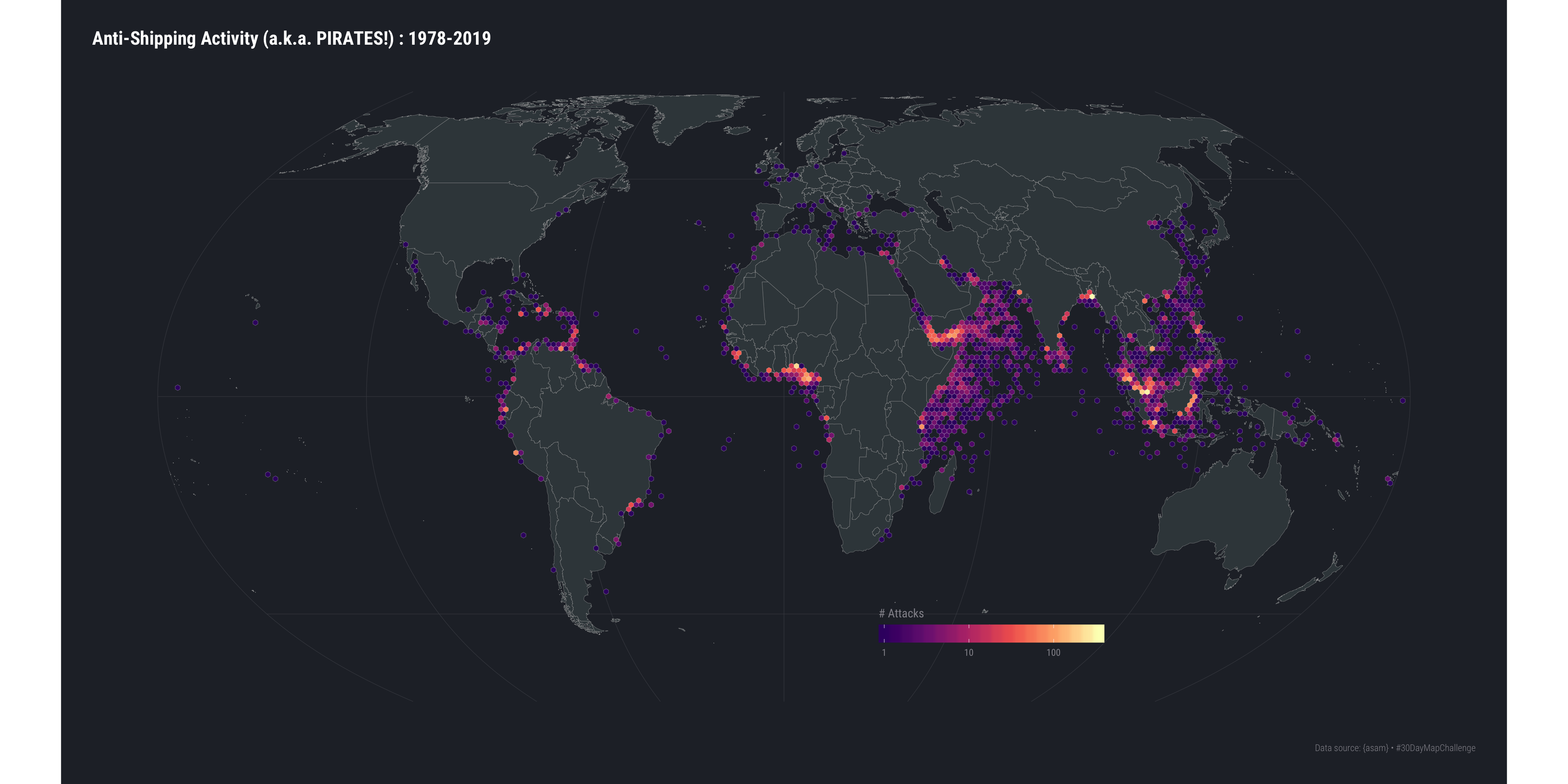
6.8 In Review
This exercise built on previous knowledge but introduced how to make your own spatial objects from data you’ve collected. It also showed how to use additional tools in the {sf} ecosystem to make a grid out of a basemap set of polygons.
6.9 Try This At Home
My original intent was to have an animated gif of pirate attacks by decade and another one of accumulated pirate attacks over those same decades. Your mission: make the animation(s)!
Much of the “decade” code is in place and even some of the labeling template code is there, too. Poke a bit about the {magick} package to see how to plot to a virtual graphics device and layer in the animations.