Skip navigation

Category Archives: Charts & Graphs

In the previous installment, a foundation was laid for “parameterizing” fonts, colors and overall slopegraph size. However, a big failing in all this code (up until now) was the reliance on character string length to determine label width. When working with fonts, the font metrics are more important since a lowercase ‘l’ will have a smaller font width than an uppercase ‘D’. So, while ‘llll’ is “longer” than ‘DDD’, it may not be wider (especially in a sans-serif font, but likely in any font):

To solve this problem, we need to use a temporary Cairo surface to compute font metrics for each label & value so we know what the maximum width of both for the starting and ending points. It’s a simple concept & calculation, but very important to ensure everything lines up well.

  1. # find the *real* maximum label width (not just based on number of chars)
  2.  
  3. maxLabelWidth = 0
  4. maxNumWidth = 0
  5.  
  6. for k in sorted(startKeys):
  7. 	s1 = starts[k]
  8. 	xbearing, ybearing, sWidth, sHeight, xadvance, yadvance = (cr.text_extents(s1))
  9. 	if (sWidth > maxLabelWidth) : maxLabelWidth = sWidth
  10. 	xbearing, ybearing, startMaxLabelWidth, startMaxLabelHeight, xadvance, yadvance = (cr.text_extents(str(k)))
  11. 	if (startMaxLabelWidth > maxNumWidth) : maxNumWidth = startMaxLabelWidth
  12.  
  13. sWidth = maxLabelWidth
  14. startMaxLabelWidth = maxNumWidth
  15.  
  16. maxWidth = 0
  17. maxNumWidth = 0
  18.  
  19. for k in sorted(endKeys):
  20. 	e1 = ends[k]
  21. 	xbearing, ybearing, eWidth, eHeight, xadvance, yadvance = (cr.text_extents(e1))
  22. 	if (eWidth > maxLabelWidth) : maxLabelWidth = eWidth
  23. 	xbearing, ybearing, endMaxLabelWidth, endMaxLabelHeight, xadvance, yadvance = (cr.text_extents(str(k)))
  24. 	if (endMaxLabelWidth > maxNumWidth) : maxNumWidth = endMaxLabelWidth
  25.  
  26. eWidth = maxLabelWidth
  27. endMaxLabelWidth = maxNumWidth

I tossed some “anomalies” into the sample data set to show both how adaptable the vertical scale is as well as demonstrate the label alignments:

Updates are in github.

On the heels of last evening’s release of Slopegraphs in Python post comes some minor tweaks:

  • Complete alignment control of labels & and values
  • Colors (for background, lines, labels & values) — I picked a random pattern from Adobe’s Kuler
  • A font change (to prove width calculations work)

…and a new example slopegraph:

As promised, the latest revisions are in github.

Some notes for aspiring Python/Cairo hackers:

  • RGB colors are 0-1 in Cairo, so divide your 0-255 values by 255 to get the corresponding Cairo value and make sure you’re doing float arithmetic in Python
  • It turns out simple Cairo font rendering (ie. non-Pango) does not interpret well in Illustrator from a Cairo PDF surface, so if you do plan on post-processing the slopegraphs, use a postscript/EPS surface:
    1. surface = cairo.PSSurface ("slopegraph.ps", width, height)
    2. surface.set_eps(True)

    (I’ll be incorporating an output option as this gets closer to 1.0)

  • If you do plan on using this at all, grab the Bitstream Vera Serif font (link goes to FontSquirrel, but you can find it almost everywhere as it’s free)

(NOTE: You can keep up with progress best at github, but can always search on “slopegraph” here or just hit the tag page: “slopegraph” regularly)

I’ve been a bit obsessed with slopegraphs (a.k.a “Tufte table-chart”) of late and very dissatisfied with the lack of tools to make this particular visualization tool more prevalent. While my ultimate goal is to have a user-friendly modern web app or platform app that’s as easy as a “drag & drop” of a CSV file, this first foray will require a bit (not much, really!) of elbow grease to be used.

For those who want to get right to the code, head on over to github and have a look (I’ll post all updates there). Setup, sample & source are also below.

First, you’ll need a modern Python install. I did all the development on Mac OS Mountain Lion (beta) with the stock Python 2.7 build. You’ll also need the Cairo 2D graphics library which built and installed perfectly from source, even on ML, so it should work fine for you. If you want something besides PDF rendering, you may need additional libraries, but PDF is decent for hi-res embedding, converting to jpg/png (see below) and tweaking in programs like Illustrator.

If you search for “Gender Comparisons” in the comments on this post at Tufte’s blog, you’ll see what I was trying to reproduce in this bit of skeleton code (below). By modifying the CSV file you’re using [line 21] and then which fields are relevant [lines 45-47] you should be able to make your own basic slopegraphs without much trouble.

If you catch any glitches, add some tweak or have a slopegraph “wish list”, let me know here, twitter (@hrbrmstr) or over at github.

  1. # slopegraph.py
  2. #
  3. # Author: Bob Rudis (@hrbrmstr)
  4. #
  5. # Basic Python skeleton to do simple two value slopegraphs
  6. # with output to PDF (most useful form for me...Cairo has tons of options)
  7. #
  8. # Find out more about & download Cairo here:
  9. # http://cairographics.org/
  10. #
  11. # 2012-05-28 - 0.5 - Initial github release. Still needs some polish
  12. #
  13.  
  14. import csv
  15. import cairo
  16.  
  17. # original data source: http://www.calvin.edu/~stob/data/television.csv
  18.  
  19. # get a CSV file to work with 
  20.  
  21. slopeReader = csv.reader(open('television.csv', 'rb'), delimiter=',', quotechar='"')
  22.  
  23. starts = {} # starting "points"/
  24. ends = {} # ending "points"
  25.  
  26. # Need to refactor label max width into font calculations
  27. # as there's no guarantee the longest (character-wise)
  28. # label is the widest one
  29.  
  30. startLabelMaxLen = 0
  31. endLabelMaxLen = 0
  32.  
  33. # build a base pair array for the final plotting
  34. # wastes memory, but simplifies plotting
  35.  
  36. pairs = []
  37.  
  38. for row in slopeReader:
  39.  
  40. 	# add chosen values (need start/end for each CSV row)
  41. 	# to the final plotting array. Try this sample with 
  42. 	# row[1] (average life span) instead of row[5] to see some
  43. 	# of the scaling in action
  44.  
  45. 	lab = row[0] # label
  46. 	beg = row[5] # male life span
  47. 	end = row[4] # female life span
  48.  
  49. 	pairs.append( (float(beg), float(end)) )
  50.  
  51. 	# combine labels of common values into one string
  52. 	# also (as noted previously, inappropriately) find the
  53. 	# longest one
  54.  
  55. 	if beg in starts:
  56. 		starts[beg] = starts[beg] + "; " + lab
  57. 	else:
  58. 		starts[beg] = lab
  59.  
  60. 	if ((len(starts[beg]) + len(beg)) > startLabelMaxLen):
  61. 		startLabelMaxLen = len(starts[beg]) + len(beg)
  62. 		s1 = starts[beg]
  63.  
  64.  
  65. 	if end in ends:
  66. 		ends[end] = ends[end] + "; " + lab
  67. 	else:
  68. 		ends[end] = lab
  69.  
  70. 	if ((len(ends[end]) + len(end)) > endLabelMaxLen):
  71. 		endLabelMaxLen = len(ends[end]) + len(end)
  72. 		e1 = ends[end]
  73.  
  74. # sort all the values (in the event the CSV wasn't) so
  75. # we can determine the smallest increment we need to use
  76. # when stacking the labels and plotting points
  77.  
  78. startSorted = [(k, starts[k]) for k in sorted(starts)]
  79. endSorted = [(k, ends[k]) for k in sorted(ends)]
  80.  
  81. startKeys = sorted(starts.keys())
  82. delta = max(startSorted)
  83. for i in range(len(startKeys)):
  84. 	if (i+1 <= len(startKeys)-1):
  85. 		currDelta = float(startKeys[i+1]) - float(startKeys[i])
  86. 		if (currDelta < delta):
  87. 			delta = currDelta
  88.  
  89. endKeys = sorted(ends.keys())
  90. for i in range(len(endKeys)):
  91. 	if (i+1 <= len(endKeys)-1):
  92. 		currDelta = float(endKeys[i+1]) - float(endKeys[i])
  93. 		if (currDelta < delta):
  94. 			delta = currDelta
  95.  
  96. # we also need to find the absolute min & max values
  97. # so we know how to scale the plots
  98.  
  99. lowest = min(startKeys)
  100. if (min(endKeys) < lowest) : lowest = min(endKeys)
  101.  
  102. highest = max(startKeys)
  103. if (max(endKeys) > highest) : highest = max(endKeys)
  104.  
  105. # just making sure everything's a number
  106. # probably should move some of this to the csv reader section
  107.  
  108. delta = float(delta)
  109. lowest = float(lowest)
  110. highest = float(highest)
  111. startLabelMaxLen = float(startLabelMaxLen)
  112. endLabelMaxLen = float(endLabelMaxLen)
  113.  
  114. # setup line width and font-size for the Cairo
  115. # you can change these and the constants should
  116. # scale the plots accordingly
  117.  
  118. FONT_SIZE = 9
  119. LINE_WIDTH = 0.5
  120.  
  121. # there has to be a better way to get a base "surface"
  122. # to do font calculations besides this. we're just making
  123. # this Cairo surface to we know the max pixel width 
  124. # (font extents) of the labels in order to scale the graph
  125. # accurately (since width/height are based, in part, on it)
  126.  
  127. filename = 'slopegraph.pdf'
  128. surface = cairo.PDFSurface (filename, 8.5*72, 11*72)
  129. cr = cairo.Context (surface)
  130. cr.save()
  131. cr.select_font_face("Sans", cairo.FONT_SLANT_NORMAL, cairo.FONT_WEIGHT_NORMAL)
  132. cr.set_font_size(FONT_SIZE)
  133. cr.set_line_width(LINE_WIDTH)
  134. xbearing, ybearing, sWidth, sHeight, xadvance, yadvance = (cr.text_extents(s1))
  135. xbearing, ybearing, eWidth, eHeight, xadvance, yadvance = (cr.text_extents(e1))
  136. xbearing, ybearing, spaceWidth, spaceHeight, xadvance, yadvance = (cr.text_extents(" "))
  137. cr.restore()
  138. cr.show_page()
  139. surface.finish()
  140.  
  141. # setup some more constants for plotting
  142. # all of these are malleable and should cascade nicely
  143.  
  144. X_MARGIN = 10
  145. Y_MARGIN = 10
  146. SLOPEGRAPH_CANVAS_SIZE = 200
  147. spaceWidth = 5
  148. LINE_HEIGHT = 15
  149. PLOT_LINE_WIDTH = 0.5
  150.  
  151. width = (X_MARGIN * 2) + sWidth + spaceWidth + SLOPEGRAPH_CANVAS_SIZE + spaceWidth + eWidth
  152. height = (Y_MARGIN * 2) + (((highest - lowest + 1) / delta) * LINE_HEIGHT)
  153.  
  154. # create the real Cairo surface/canvas
  155.  
  156. filename = 'slopegraph.pdf'
  157. surface = cairo.PDFSurface (filename, width, height)
  158. cr = cairo.Context (surface)
  159.  
  160. cr.save()
  161.  
  162. cr.select_font_face("Sans", cairo.FONT_SLANT_NORMAL, cairo.FONT_WEIGHT_NORMAL)
  163. cr.set_font_size(FONT_SIZE)
  164.  
  165. cr.set_line_width(LINE_WIDTH)
  166. cr.set_source_rgba (0, 0, 0) # need to make this a constant
  167.  
  168. # draw start labels at the correct positions
  169. # cheating a bit here as the code doesn't (yet) line up 
  170. # the actual data values
  171.  
  172. for k in sorted(startKeys):
  173.  
  174. 	label = starts[k]
  175. 	xbearing, ybearing, lWidth, lHeight, xadvance, yadvance = (cr.text_extents(label))
  176.  
  177. 	val = float(k)
  178.  
  179. 	cr.move_to(X_MARGIN + (sWidth - lWidth), Y_MARGIN + (highest - val) * LINE_HEIGHT * (1/delta) + LINE_HEIGHT/2)
  180. 	cr.show_text(label + " " + k)
  181. 	cr.stroke()
  182.  
  183. # draw end labels at the correct positions
  184. # cheating a bit here as the code doesn't (yet) line up 
  185. # the actual data values
  186.  
  187. for k in sorted(endKeys):
  188.  
  189. 	label = ends[k]
  190. 	xbearing, ybearing, lWidth, lHeight, xadvance, yadvance = (cr.text_extents(label))
  191.  
  192. 	val = float(k)
  193.  
  194. 	cr.move_to(width - X_MARGIN - eWidth - (4*spaceWidth), Y_MARGIN + (highest - val) * LINE_HEIGHT * (1/delta) + LINE_HEIGHT/2)
  195. 	cr.show_text(k + " " + label)
  196. 	cr.stroke()
  197.  
  198. # do the actual plotting
  199.  
  200. cr.set_line_width(PLOT_LINE_WIDTH)
  201. cr.set_source_rgba (0.75, 0.75, 0.75) # need to make this a constant
  202.  
  203. for s1,e1 in pairs:
  204. 	cr.move_to(X_MARGIN + sWidth + spaceWidth + 20, Y_MARGIN + (highest - s1) * LINE_HEIGHT * (1/delta) + LINE_HEIGHT/2)
  205. 	cr.line_to(width - X_MARGIN - eWidth - spaceWidth - 20, Y_MARGIN + (highest - e1) * LINE_HEIGHT * (1/delta) + LINE_HEIGHT/2)
  206. 	cr.stroke()
  207.  
  208. cr.restore()
  209. cr.show_page()
  210. surface.finish()

I didn’t read through the Massachusetts 2011 Report on Data Breach Notifications [PDF] until recently, but once I went through the report my brain kept telling me “something is wrong”. Not something earth shattering, but more of a “something is off” signal. This happens more than I’d like as I tend to constantly background process what I intake visually.

As Twitter followers may lament, I have been known to transcribe useful tabular information from reports such as these, especially when I need to communicate them internally and I have done so with this report [gdocs] as well.

After working through the whole document, the last page of data is where I found the “off by one” error (see figure below). Someone performed “head math” vs copying & formatting from a spreadsheet. Never a good idea if you aren’t going to double-check the report thoroughly.


Off By One

My transcription (“Lost Stolen Misplaced” tab in the aforelinked workbook) assumes the “5” and “48” are correct and has the correct total (“53”). One of the problems when an error like this crops up is that you do not know where the error occurred, but since the sums of “12” and “277” are both correct in the spreadsheet and in the report, I think I’ve found the culprit. Unfortunately, a computational error such as this does foster suspicion on the accuracy of the rest of the report data.

It’s a lesson report writers should heed well: compute twice, publish once. Errant data can cut as deeply as a saw blade.

While I Have Your Attention

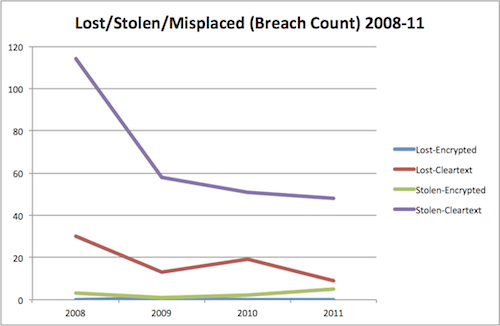
Since there aren’t many visualizations in  Massachusetts 2011 Report on Data Breach Notifications (3D numbers do not count), here are a few I made that I found helpful during my interpretation (2011 data unless otherwise specified):

# Residents Impacted By Breah Org

Number Of Breached By Org

Number of Breaches by Type 2008-2011

Residents Impacted By Breach Type

Lost/Stolen/Misplaced

Malicious/Non-Malicious


As promised, this post is a bit more graphical, but I feel the need to stress the importance of the first few points in chapter 2 of the book (i.e. the difference between mean and average and why variance is meaningful). These are fundamental concepts for future work.

The “pumpkin” example (2.1) gives us an opportunity to do some very basic R:

  1. pumpkins <- c(1,1,1,3,3,591) #build an array
  2. mean(pumpkins) #mean (average)
  3. var(pumpkins) #variance
  4. sd(pumpkins) #deviation

(as you can see, I’m still trying to find the best way to embed R source code)

We move from pumpkins to babies for Example 2.2 (you’ll need the whole bit of source from previous examples (that includes all the solutions in this example) to make the rest of the code snippets work). Here, we can quickly compute and compare the standard deviations (with difference) and the means (with difference) to help us analyze the statistical significane questions in the chapter:

  1. sd(firstbabies$prglength)
  2. sd(notfirstbabies$prglength)
  3. sd(firstbabies$prglength) - sd(notfirstbabies$prglength)
  4.  
  5. mean(firstbabies$prglength)
  6. mean(notfirstbabies$prglength)
  7. mean(firstbabies$prglength) - mean(notfirstbabies$prglength)

You’ll see the power of R’s hist function in a moment, but you should be a bit surprised when you see the output if you enter to solve Example 2.3:

  1. mode(firstbabies$prglength)

That’s right, R does not have a built-in mode function. It’s pretty straightforward to compute, tho:

  1. names(sort(-table(firstbabies$prglength))[1])

(notice how “straightforward” != “simple”)

We have to use the table function to generate a table of value frequencies. It’s a two-dimensional structure with the actual value associated with the frequency represented as a string indexed at the same position. Using “-” inverts all the values (but keeps the two-dimensional indexing consistent) and sort orders the structure so we can use index “[1]” to get to the value we’re looking for. By using the names function, we get the string representing the value at the highest frequency. You can see this iteratively by breaking out the code:

  1. table(firstbabies$prglength)
  2. str(table(firstbabies$prglength))
  3. sort(table(firstbabies$prglength))
  4. sort(table(firstbabies$prglength))[1] #without the "-"
  5. sort(-table(firstbabies$prglength))[1]
  6. names(sort(-table(firstbabies$prglength))[1])

There are a plethora of other ways to compute the mode, but this one seems to work well for my needs.

Pictures Or It Didn’t Happen

I did debate putting the rest of this post into a separate example, but if you’ve stuck through this far, you deserve some stats candy. It’s actually pretty tricky to do what the book does here:

So, we’ll start off with simple histogram plots of each set being compared:

  1. hist(firstbabies$prglength)

  1. hist(notfirstbabies$prglength)

I separated those out since hist by default displays the histogram and if you just paste the lines consecutively, you’ll only see the last histogram. What does display is, well, ugly and charts should be beautiful. It will take a bit to explain the details (in another post) but this should get you started:

  1. par(mfrow=c(1,2))par(mfrow=c(1,2))
  2. hist(firstbabies$prglength, cex.lab=0.8, cex.axis=0.6, cex.main=0.8, las=1, col="white", ylim=c(0,3000),xlim=c(17,max(firstbabies$prglength)), breaks="Scott", main="Histogram of first babies", xlab="Weeks")
  3. hist(notfirstbabies$prglength, cex.lab=0.8, cex.axis=0.6, cex.main=0.8, las=1, col="blue", ylim=c(0,3000),xlim=c(17,max(notfirstbabies$prglength)), breaks="Scott", main="Histogram of other babies", xlab="Weeks")
  4. par(mfrow=c(1,1))

In the above code, we’re telling R to setup a canvas that will have one row and two plot areas. This makes it very easy to have many graphs on one canvas.

Next, the first hist sets up up some label proportions (the cex parameters), tells R to make Y labels horizontal (las=1), makes the bars white, sets up sane values for the X & Y axes, instructs R to use the “Scott” algorithm for calculating sane bins (we’ll cover this in more details next post) and sets up sane titles and X axis labels. Finally, we reset the canvas for the next plot.

There’s quite a bit to play with there and you can use the “help()” command to get information on the hist function and plot function. You can setup your own bin size by substituting an array for “Scott”. If you have specific questions, shoot a note in the comments, but I’ll explain more about what’s going on in the next post as we add in probability histograms and start looking at the data in more detail.


Click for larger image

Download R Source of Examples 2.1-2.3

I wanted to play with the AwesomeChartJS library and figured an interesting way to do that was to use it to track Microsoft Security Bulletins this year. While I was drawn in by just how simple it is to craft basic charts, that simplicity really only makes it useful for simple data sets. So, while I’ve produced three diferent views of Microsoft Security Bulletins for 2011 (to-date, and in advance of February’s Patch Tuesday), it would not be a good choice to do a running comparison between past years and 20111 (per-month).  The authors self-admit that there are [deliberate] limitations and point folks to the most excellent flot library for more sophisticated analytics (which I may feature in March).

The library itself only works within an HTML5 environment (one of the reasons I chose it) and uses a separate <canvas> element to house each chart. After loading up the library iself in a script tag:

<script src="/b/js/AwesomeChartJS/awesomechart.js" type="application/javascript">

(which is ~32K un-minified) you then declare a canvas element:

<canvas id="canvas1" width="400" height="300"></canvas>


and use some pretty straighforward javascript (no dependency on jQuery or other large frameworks) to do the drawing:

var mychart = new AwesomeChart('canvas1');
mychart.title = "Microsoft Security Bulletins Raw Count By Month - 2011";
mychart.data = [2, 12];
mychart.colors = ["#0000FF","#0000FF"];
mychart.labels = ["January", "February"];
mychart.draw();

It’s definitely worth a look if you have simple charting needs.

Regrettably, it looks like February is going to be a busy month for Windows administrators.

Your web-browser does not support the HTML 5 canvas element.

Your web-browser does not support the HTML 5 canvas element.

Your web-browser does not support the HTML 5 canvas element.