The @pewresearch folks have been collecting political survey data for quite a while, and I noticed the visualization below referenced in a Tableau vis contest entry:
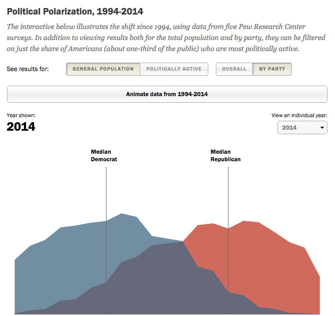
Those are filled frequency polygons, which are super-easy to replicate in ggplot2, especially since Pew even kind of made the data available via their interactive visualization (it’s available in other Pew resources, just not as compact). So, we can look at all 5 study years for both the general population and politically active respondents with ggplot2 facets, incorporating the use of V8, dplyr, tidyr, purrr and some R spatial functions along the way.
The first code block has the “data”, data transformations and initial plot code. The “data” is really javascript blocks picked up from the view-source: of the interactive visualization. We use the V8 package to get this data then bend it to our will for visuals.
library(V8)
library(dplyr)
library(tidyr)
library(purrr)
library(ggplot2)  # devtools::install_github("hadley/ggplot2)
library(hrbrmisc) # devtools::install_github("hrbrmstr/hrbrmisc)
library(rgeos)
library(sp)

ctx <- v8()
ctx$eval("
	var party_data = [
		[{
			name: 'Dem',
			data: [0.57,1.60,1.89,3.49,3.96,6.56,7.23,8.54,9.10,9.45,9.30,9.15,7.74,6.80,4.66,4.32,2.14,1.95,0.87,0.57,0.12]
		},{
			name: 'REP',
			data: [0.03,0.22,0.28,1.49,1.66,2.77,3.26,4.98,5.36,7.28,7.72,8.16,8.86,8.88,8.64,8.00,6.20,5.80,4.87,4.20,1.34]
		}],
		[{
			name: 'Dem',
			data: [1.22,2.78,3.28,5.12,6.15,7.77,8.24,9.35,9.73,9.19,8.83,8.47,5.98,5.17,3.62,2.87,1.06,0.75,0.20,0.15,0.04]
		}, {
			name: 'REP',
			data: [0.23,0.49,0.65,2.23,2.62,4.06,5.02,7.53,7.70,7.28,7.72,8.15,8.87,8.47,7.08,6.27,4.29,3.99,3.54,2.79,1.03]
		}],
		[{
			name: 'Dem',
			data: [2.07,3.57,4.21,6.74,7.95,8.41,8.58,9.07,8.98,8.46,8.47,8.49,5.39,3.62,2.11,1.98,1.00,0.55,0.17,0.17,0.00]
		}, {
			name: 'REP',
			data: [0.19,0.71,1.04,2.17,2.07,3.65,4.92,7.28,8.26,9.64,9.59,9.55,7.91,7.74,6.84,6.01,4.37,3.46,2.09,1.65,0.86]
		}],
		[{
			name: 'Dem',
			data: [2.97,4.09,4.28,6.65,7.90,8.37,8.16,8.74,8.61,8.15,7.74,7.32,4.88,4.82,2.79,2.07,0.96,0.78,0.41,0.29,0.02]
		}, {
			name: 'REP',
			data: [0.04,0.21,0.28,0.88,1.29,2.64,3.08,4.92,5.84,6.65,6.79,6.92,8.50,8.61,8.05,8.00,7.52,7.51,5.61,4.17,2.50]
		}],
		[{
			name: 'Dem',
			data: [4.81,6.04,6.57,7.67,7.84,8.09,8.24,8.91,8.60,6.92,6.69,6.47,4.22,3.85,1.97,1.69,0.66,0.49,0.14,0.10,0.03]
		}, {
			name: 'REP',
			data: [0.11,0.36,0.49,1.23,1.35,2.35,2.83,4.63,5.09,6.12,6.27,6.41,7.88,8.03,7.58,8.26,8.12,7.29,6.38,5.89,3.34]
		}],
	];

	var party_engaged_data = [
		[{
			name: 'Dem',
			data: [0.88,2.19,2.61,4.00,4.76,6.72,7.71,8.45,8.03,8.79,8.79,8.80,7.23,6.13,4.53,4.31,2.22,2.01,1.05,0.66,0.13]
		}, {
			name: 'REP',
			data: [0.00,0.09,0.09,0.95,1.21,1.67,2.24,3.22,3.70,6.24,6.43,6.62,8.01,8.42,8.97,8.48,7.45,7.68,8.64,7.37,2.53]
		}],
		[{
			name: 'Dem',
			data: [1.61,3.35,4.25,6.75,8.01,8.20,8.23,9.14,8.94,8.68,8.46,8.25,4.62,3.51,2.91,2.63,1.19,0.74,0.24,0.17,0.12]
		},{
			name: 'REP',
			data: [0.21,0.38,0.68,1.62,1.55,2.55,3.99,4.65,4.31,5.78,6.28,6.79,8.47,9.01,8.61,8.34,7.16,6.50,6.10,4.78,2.25]
		}],
		[{
			name: 'Dem',
			data: [3.09,4.89,6.22,9.40,9.65,9.20,8.99,6.48,7.36,7.67,6.95,6.22,4.53,3.79,2.19,2.02,0.74,0.07,0.27,0.27,0.00]
		}, {
			name: 'REP',
			data: [0.29,0.59,0.67,2.11,2.03,2.67,4.12,6.55,6.93,8.42,8.79,9.17,7.33,6.84,7.42,7.25,6.36,5.32,3.35,2.57,1.24]
		}],
		[{
			name: 'Dem',
			data: [6.00,5.24,5.11,7.66,9.25,8.25,8.00,8.09,8.12,7.05,6.59,6.12,4.25,4.07,2.30,1.49,0.98,0.80,0.42,0.16,0.06]
		}, {
			name: 'REP',
			data: [0.00,0.13,0.13,0.48,0.97,2.10,2.73,3.14,3.64,5.04,5.30,5.56,6.87,6.75,8.03,9.33,11.01,10.49,7.61,6.02,4.68]
		}],
		[{
			name: 'Dem',
			data: [9.53,9.68,10.35,9.33,9.34,7.59,6.67,6.41,6.60,5.21,4.84,4.47,2.90,2.61,1.37,1.14,0.73,0.59,0.30,0.28,0.06]
		}, {
			name: 'REP',
			data: [0.15,0.11,0.13,0.46,0.52,1.18,1.45,2.46,2.84,4.15,4.37,4.60,6.36,6.66,7.34,9.09,11.40,10.53,10.58,9.85,5.76]
		}],
	];
")

years <- c(1994, 1999, 2004, 2001, 2014)

# Transform the javascript data -------------------------------------------

party_data <- ctx$get("party_data")
map_df(1:length(party_data), function(i) {
  x <- party_data[[i]]
  names(x$data) <- x$name
  dat <- as.data.frame(x$data)
  bind_cols(dat, data_frame(x=-10:10, year=rep(years[i], nrow(dat))))
}) -> party_data

party_engaged_data <- ctx$get("party_engaged_data")
map_df(1:length(party_engaged_data), function(i) {
  x <- party_engaged_data[[i]]
  names(x$data) <- x$name
  dat <- as.data.frame(x$data)
  bind_cols(dat, data_frame(x=-10:10, year=rep(years[i], nrow(dat))))
}) -> party_engaged_data

# We need it in long form -------------------------------------------------

gather(party_data, party, pct, -x, -year) %>%
  mutate(party=factor(party, levels=c("REP", "Dem"))) -> party_data_long

gather(party_engaged_data, party, pct, -x, -year) %>%
  mutate(party=factor(party, levels=c("REP", "Dem"))) -> party_engaged_data_long

# Traditional frequency polygon plots -------------------------------------

gg <- ggplot()
gg <- gg + geom_ribbon(data=party_data_long,
                       aes(x=x, ymin=0, ymax=pct, fill=party, color=party), alpha=0.5)
gg <- gg + scale_x_continuous(expand=c(0,0), breaks=c(-8, 0, 8),
                              labels=c("Consistently\nliberal", "Mixed", "Consistently\nconservative"))
gg <- gg + scale_y_continuous(expand=c(0,0), limits=c(0, 12))
gg <- gg + scale_color_manual(name=NULL, values=c(Dem="#728ea2", REP="#cf6a5d"),
                              labels=c(Dem="Democrats", REP="Republicans"))
gg <- gg + guides(color="none", fill=guide_legend(override.aes=list(alpha=1)))
gg <- gg + scale_fill_manual(name=NULL, values=c(Dem="#728ea2", REP="#cf6a5d"),
                             labels=c(Dem="Democrats", REP="Republicans"))
gg <- gg + facet_wrap(~year, ncol=2, scales="free_x")
gg <- gg + labs(x=NULL, y=NULL,
                title="Political Polarization, 1994-2014 (General Population)",
                caption="Source: http://www.people-press.org/2014/06/12/section-1-growing-ideological-consistency/iframe/")
gg <- gg + theme_hrbrmstr_an(grid="")
gg <- gg + theme(panel.margin=margin(t=30, b=30, l=30, r=30))
gg <- gg + theme(legend.position=c(0.75, 0.1))
gg <- gg + theme(legend.direction="horizontal")
gg <- gg + theme(axis.text.y=element_blank())
gg

gg <- ggplot()
gg <- gg + geom_ribbon(data=party_engaged_data_long,
                       aes(x=x, ymin=0, ymax=pct, fill=party, color=party), alpha=0.5)
gg <- gg + scale_x_continuous(expand=c(0,0), breaks=c(-8, 0, 8),
                              labels=c("Consistently\nliberal", "Mixed", "Consistently\nconservative"))
gg <- gg + scale_y_continuous(expand=c(0,0), limits=c(0, 12))
gg <- gg + scale_color_manual(name=NULL, values=c(Dem="#728ea2", REP="#cf6a5d"),
                              labels=c(Dem="Democrats", REP="Republicans"))
gg <- gg + guides(color="none", fill=guide_legend(override.aes=list(alpha=1)))
gg <- gg + scale_fill_manual(name=NULL, values=c(Dem="#728ea2", REP="#cf6a5d"),
                             labels=c(Dem="Democrats", REP="Republicans"))
gg <- gg + facet_wrap(~year, ncol=2, scales="free_x")
gg <- gg + labs(x=NULL, y=NULL,
                title="Political Polarization, 1994-2014 (Politically Active)",
                caption="Source: http://www.people-press.org/2014/06/12/section-1-growing-ideological-consistency/iframe/")
gg <- gg + theme_hrbrmstr_an(grid="")
gg <- gg + theme(panel.margin=margin(t=30, b=30, l=30, r=30))
gg <- gg + theme(legend.position=c(0.75, 0.1))
gg <- gg + theme(legend.direction="horizontal")
gg <- gg + theme(axis.text.y=element_blank())
gg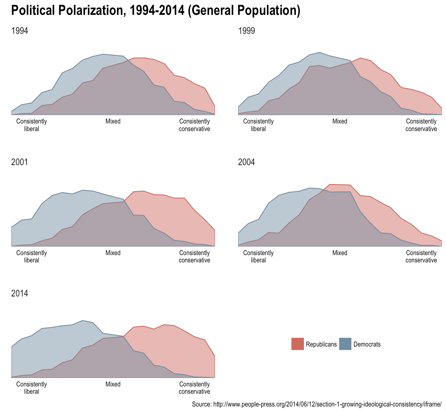
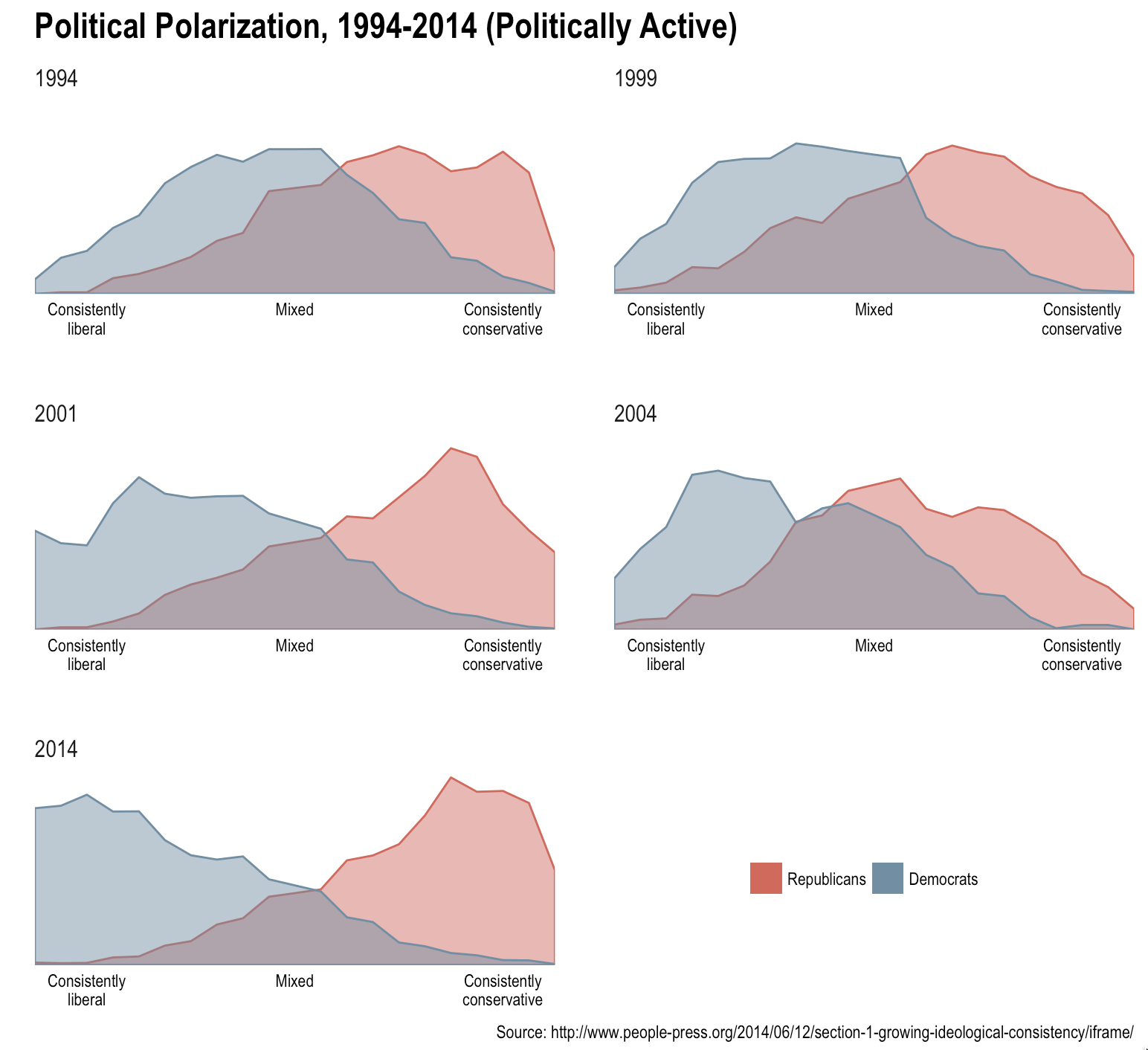
It provides a similar effect to the Pew & Interworks visuals using alpha transparency to blend the point of polygon intersections. But I really kinda like the way both Pew & Interworks did their visualizations without alpha blending yet still highlighting the intersected areas. We can do that in R as well with a bit more work by:
- grouping each data frame by year
- turning each set of points (Dem & Rep) to R polygons
- computing the intersection of those polygons
- turning that intersection back into a data frame
- adding this new polygon to the plots while also removing the alpha blend
Here’s what that looks like in code:
# Setup a function to do the polygon intersection -------------------------

polysect <- function(df) {

  bind_rows(data_frame(x=-10, pct=0),
            select(filter(df, party=="Dem"), x, pct),
            data_frame(x=10, pct=0)) %>%
    as.matrix() %>%
    Polygon() %>%
    list() %>%
    Polygons(1) %>%
    list() %>%
    SpatialPolygons() -> dem

  bind_rows(data_frame(x=-10, pct=0),
            select(filter(df, party=="REP"), x, pct),
            data_frame(x=10, pct=0)) %>%
    as.matrix() %>%
    Polygon() %>%
    list() %>%
    Polygons(1) %>%
    list() %>%
    SpatialPolygons() -> rep

  inter <- gIntersection(dem, rep)
  inter <- as.data.frame(inter@polygons[[1]]@Polygons[[1]]@coords)[c(-1, -25),]
  inter <- mutate(inter, year=df$year[1])
  inter

}

# Get the intersected area ------------------------------------------------

group_by(party_data_long, year) %>%
  do(polysect(.)) -> general_sect

group_by(party_engaged_data_long, year) %>%
  do(polysect(.)) -> engaged_sect


# Try the plots again -----------------------------------------------------

gg <- ggplot()
gg <- gg + geom_ribbon(data=party_data_long,
                       aes(x=x, ymin=0, ymax=pct, fill=party, color=party))
gg <- gg + geom_ribbon(data=general_sect, aes(x=x, ymin=0, ymax=y), color="#666979", fill="#666979")
gg <- gg + scale_x_continuous(expand=c(0,0), breaks=c(-8, 0, 8),
                              labels=c("Consistently\nliberal", "Mixed", "Consistently\nconservative"))
gg <- gg + scale_y_continuous(expand=c(0,0), limits=c(0, 12))
gg <- gg + scale_color_manual(name=NULL, values=c(Dem="#728ea2", REP="#cf6a5d"),
                              labels=c(Dem="Democrats", REP="Republicans"))
gg <- gg + guides(color="none", fill=guide_legend(override.aes=list(alpha=1)))
gg <- gg + scale_fill_manual(name=NULL, values=c(Dem="#728ea2", REP="#cf6a5d"),
                             labels=c(Dem="Democrats", REP="Republicans"))
gg <- gg + facet_wrap(~year, ncol=2, scales="free_x")
gg <- gg + labs(x=NULL, y=NULL,
                title="Political Polarization, 1994-2014 (General Population)",
                caption="Source: http://www.people-press.org/2014/06/12/section-1-growing-ideological-consistency/iframe/")
gg <- gg + theme_hrbrmstr_an(grid="")
gg <- gg + theme(panel.margin=margin(t=30, b=30, l=30, r=30))
gg <- gg + theme(legend.position=c(0.75, 0.1))
gg <- gg + theme(legend.direction="horizontal")
gg <- gg + theme(axis.text.y=element_blank())
gg

gg <- ggplot()
gg <- gg + geom_ribbon(data=party_engaged_data_long,
                       aes(x=x, ymin=0, ymax=pct, fill=party, color=party))
gg <- gg + geom_ribbon(data=engaged_sect, aes(x=x, ymin=0, ymax=y), color="#666979", fill="#666979")
gg <- gg + scale_x_continuous(expand=c(0,0), breaks=c(-8, 0, 8),
                              labels=c("Consistently\nliberal", "Mixed", "Consistently\nconservative"))
gg <- gg + scale_y_continuous(expand=c(0,0), limits=c(0, 12))
gg <- gg + scale_color_manual(name=NULL, values=c(Dem="#728ea2", REP="#cf6a5d"),
                              labels=c(Dem="Democrats", REP="Republicans"))
gg <- gg + guides(color="none", fill=guide_legend(override.aes=list(alpha=1)))
gg <- gg + scale_fill_manual(name=NULL, values=c(Dem="#728ea2", REP="#cf6a5d"),
                             labels=c(Dem="Democrats", REP="Republicans"))
gg <- gg + facet_wrap(~year, ncol=2, scales="free_x")
gg <- gg + labs(x=NULL, y=NULL,
                title="Political Polarization, 1994-2014 (Politically Active)",
                caption="Source: http://www.people-press.org/2014/06/12/section-1-growing-ideological-consistency/iframe/")
gg <- gg + theme_hrbrmstr_an(grid="")
gg <- gg + theme(panel.margin=margin(t=30, b=30, l=30, r=30))
gg <- gg + theme(legend.position=c(0.75, 0.1))
gg <- gg + theme(legend.direction="horizontal")
gg <- gg + theme(axis.text.y=element_blank())
gg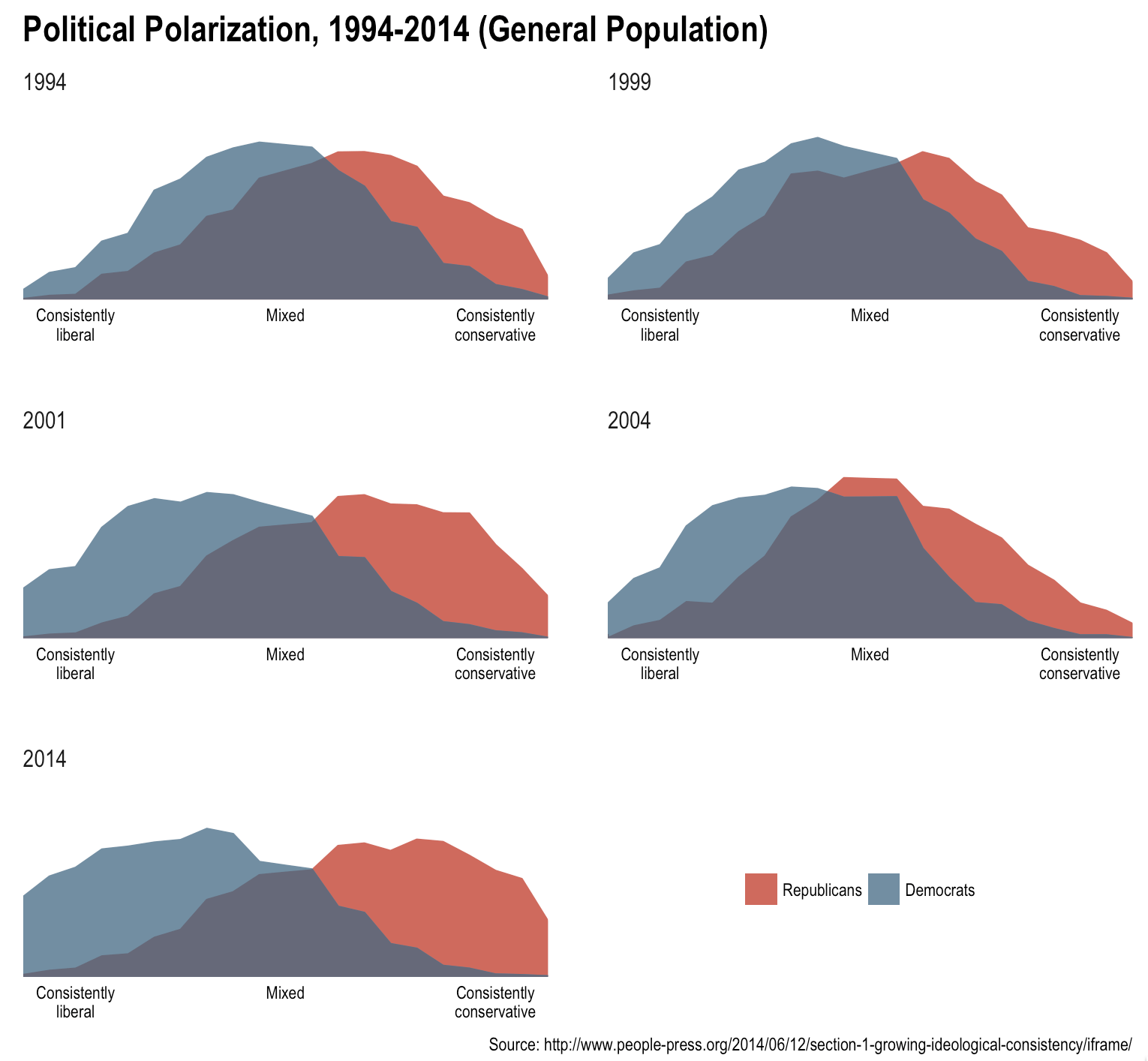
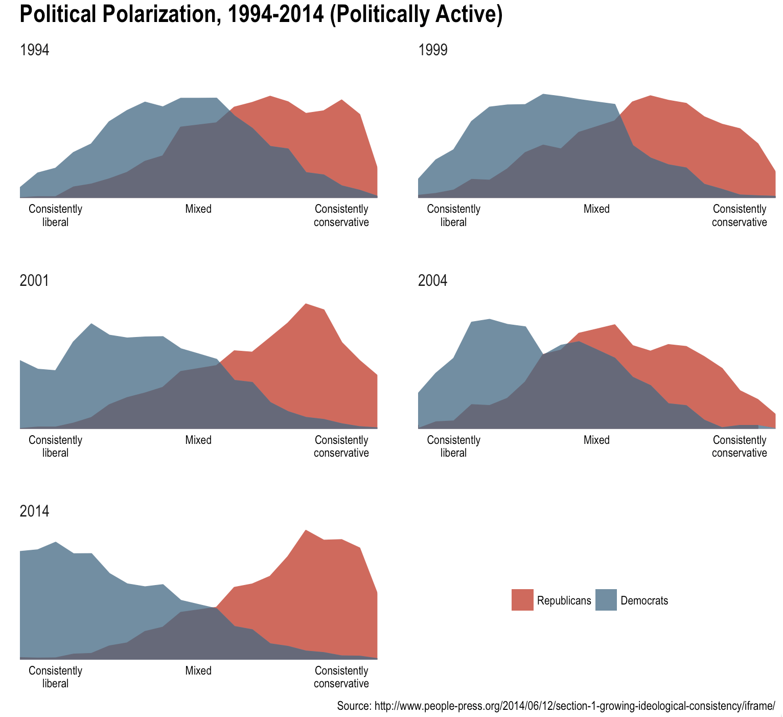
Without much extra effort/work we now have what I believe to be a more striking set of visuals. (And, I should probably makes a points_to_spatial_polys() convenience function.)
You’ll find the “overall” group data as well as the party median values in the Pew HTML source code if you want to try to fully replicate their visualizations.
No comments yet.