Chapter 1 Demystifying ggplot2
The ggplot2 system is elegant and expressive…once you finally wrap your head around it. For many, there’s a steep learning curve to ggplot2 and that learning curve often creates an aire of mysticism around what exactly goes on behind the scenes that ends up producing the magical creations that are ggplot2 visualizations.
Now, there’s an entire book by Hadley on ggplot2 and scads of other books written by others on ggplot2. This chapter is not going to cover ggplot2 in the same way. Rather, the goal, here, is to give you a sense of what goes on at a lower-level when you create a plot to help illumniate what you’ll be doing when you start building Geoms, Stats and other core ggplot2 objects.
1.1 Breaking down the seminal example
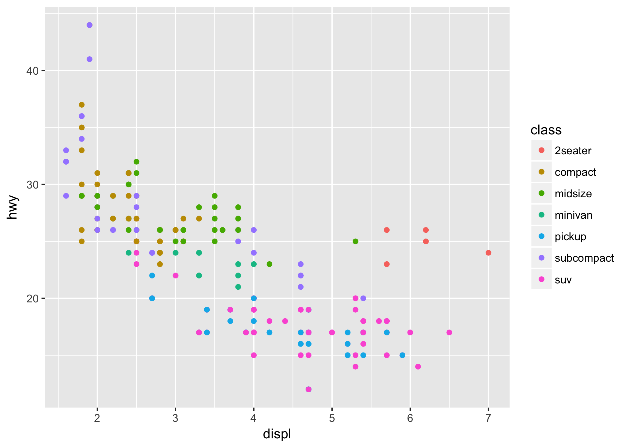
There is a classic (seminal) example plot which budding ggplot2 enthusiasts meet as their first foray into the grammar of graphics and that most regular users of ggplot2 can produce at-will from memory:

As a ggplot2 user, you know that:
- a data frame was passed in
xandyaesthetics were mapped to specific data frame columns- there is an intent to color whatever shape is being used by the contents of the
classcolumn - the desired shape to use is a point.
But, what does that code really do?
Before delving into that, though, you may not even be aware that ggplot2 filled in a bunch of missing information for you. Here’s (for the most part) what was done for you:
ggplot(mpg, aes(displ, hwy, colour = class)) +
  geom_point(stat = "identity", position = "identity", shape = 19, size = 1.5) +
  scale_x_continuous(trans = "identity") +
  scale_y_continuous(trans = "identity") +
  scale_color_hue() +
  coord_cartesian() +
  facet_null() +
  theme_gray()
After analyzing the input data and aesthetic mappings, ggplot2 is able to “automagically” determine whether to use discrete or continuous scales for various mapped values and sets a number of other critical components from sensible, thoughtful defaults. This “magic” helps reduce typing and enables you to focus on customizing only what is absolutely necessary to convey the story you’re trying to tell with the visualization.
There is one missing line from that code sequence: print().
By default, R prints evaluated objects and all you’ve done before printing is create a small, fairly complex ggplot-classed object with good intentions.
The ggplot2::print.ggplot2() function takes these intentions and transorms them — with the aid of ggplot_build() and ggplot_gtable() — into larger and even more complex structures, which are ultimately transformed into (hopefully) pretty pictures.
Examining these objects will help you get a feel for what you’ll ultimately be doing inside your own customized ggplot2 object.
1.2 The ggplot object
The first object to explore is the ggplot object itself. To that end, assign a plot to a variable and examine the structure with str()
## List of 9
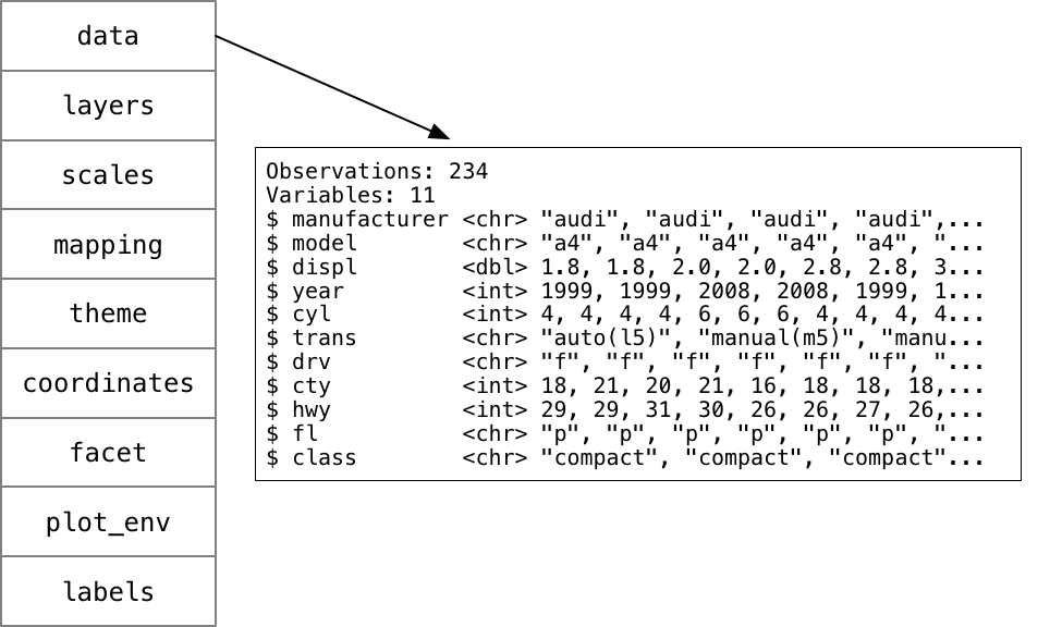
## $ data :Classes 'tbl_df', 'tbl' and 'data.frame': 234 obs. of 11 variables:
## ..$ manufacturer: chr [1:234] "audi" "audi" "audi" "audi" ...
## ..$ model : chr [1:234] "a4" "a4" "a4" "a4" ...
## ..$ displ : num [1:234] 1.8 1.8 2 2 2.8 2.8 3.1 1.8 1.8 2 ...
## ..$ year : int [1:234] 1999 1999 2008 2008 1999 1999 2008 1999 1999 2008 ...
## ..$ cyl : int [1:234] 4 4 4 4 6 6 6 4 4 4 ...
## ..$ trans : chr [1:234] "auto(l5)" "manual(m5)" "manual(m6)" "auto(av)" ...
## ..$ drv : chr [1:234] "f" "f" "f" "f" ...
## ..$ cty : int [1:234] 18 21 20 21 16 18 18 18 16 20 ...
## ..$ hwy : int [1:234] 29 29 31 30 26 26 27 26 25 28 ...
## ..$ fl : chr [1:234] "p" "p" "p" "p" ...
## ..$ class : chr [1:234] "compact" "compact" "compact" "compact" ...
## $ layers :List of 1
## ..$ :Classes 'LayerInstance', 'Layer', 'ggproto', 'gg' <ggproto object: Class LayerInstance, Layer, gg>
## aes_params: list
## compute_aesthetics: function
## compute_geom_1: function
## compute_geom_2: function
## compute_position: function
## compute_statistic: function
## data: waiver
## draw_geom: function
## finish_statistics: function
## geom: <ggproto object: Class GeomPoint, Geom, gg>
## aesthetics: function
## default_aes: uneval
## draw_group: function
## draw_key: function
## draw_layer: function
## draw_panel: function
## extra_params: na.rm
## handle_na: function
## non_missing_aes: size shape colour
## optional_aes:
## parameters: function
## required_aes: x y
## setup_data: function
## use_defaults: function
## super: <ggproto object: Class Geom, gg>
## geom_params: list
## inherit.aes: TRUE
## layer_data: function
## map_statistic: function
## mapping: NULL
## position: <ggproto object: Class PositionIdentity, Position, gg>
## compute_layer: function
## compute_panel: function
## required_aes:
## setup_data: function
## setup_params: function
## super: <ggproto object: Class Position, gg>
## print: function
## show.legend: NA
## stat: <ggproto object: Class StatIdentity, Stat, gg>
## aesthetics: function
## compute_group: function
## compute_layer: function
## compute_panel: function
## default_aes: uneval
## extra_params: na.rm
## finish_layer: function
## non_missing_aes:
## parameters: function
## required_aes:
## retransform: TRUE
## setup_data: function
## setup_params: function
## super: <ggproto object: Class Stat, gg>
## stat_params: list
## subset: NULL
## super: <ggproto object: Class Layer, gg>
## $ scales :Classes 'ScalesList', 'ggproto', 'gg' <ggproto object: Class ScalesList, gg>
## add: function
## clone: function
## find: function
## get_scales: function
## has_scale: function
## input: function
## n: function
## non_position_scales: function
## scales: list
## super: <ggproto object: Class ScalesList, gg>
## $ mapping :List of 3
## ..$ x : symbol displ
## ..$ y : symbol hwy
## ..$ colour: symbol class
## $ theme : list()
## $ coordinates:Classes 'CoordCartesian', 'Coord', 'ggproto', 'gg' <ggproto object: Class CoordCartesian, Coord, gg>
## aspect: function
## default: TRUE
## distance: function
## expand: TRUE
## is_linear: function
## labels: function
## limits: list
## modify_scales: function
## range: function
## render_axis_h: function
## render_axis_v: function
## render_bg: function
## render_fg: function
## setup_data: function
## setup_layout: function
## setup_panel_params: function
## setup_params: function
## transform: function
## super: <ggproto object: Class CoordCartesian, Coord, gg>
## $ facet :Classes 'FacetNull', 'Facet', 'ggproto', 'gg' <ggproto object: Class FacetNull, Facet, gg>
## compute_layout: function
## draw_back: function
## draw_front: function
## draw_labels: function
## draw_panels: function
## finish_data: function
## init_scales: function
## map_data: function
## params: list
## setup_data: function
## setup_params: function
## shrink: TRUE
## train_scales: function
## vars: function
## super: <ggproto object: Class FacetNull, Facet, gg>
## $ plot_env :<environment: R_GlobalEnv>
## $ labels :List of 3
## ..$ x : chr "displ"
## ..$ y : chr "hwy"
## ..$ colour: chr "class"
## - attr(*, "class")= chr [1:2] "gg" "ggplot"Yikes! Perhaps it would be better to examine that in a bit more of a deliberate fashion.
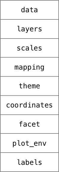
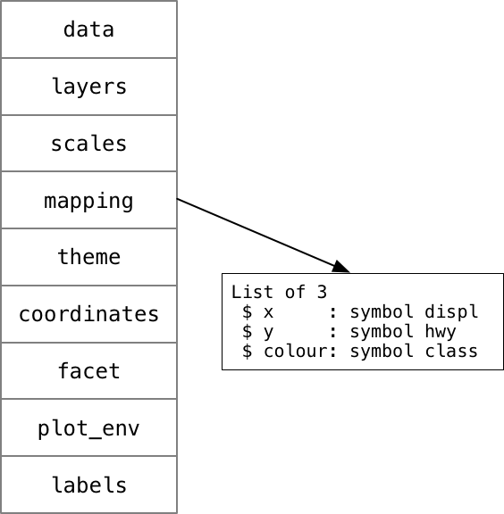
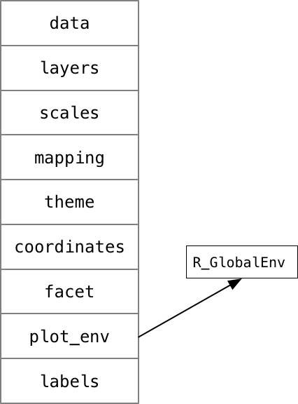
There are 9 elements in the list that make up the ggplot-classed object:
The data element is what was passed in as data to ggplot():
The layers element is a length 1 list of ggproto objects (which are the building blocks you’ll be eventually creating). There is quite a bit of (for now) extraneous internal ggproto object information cluttering up the structure display, but it can be print()ed more compactly:
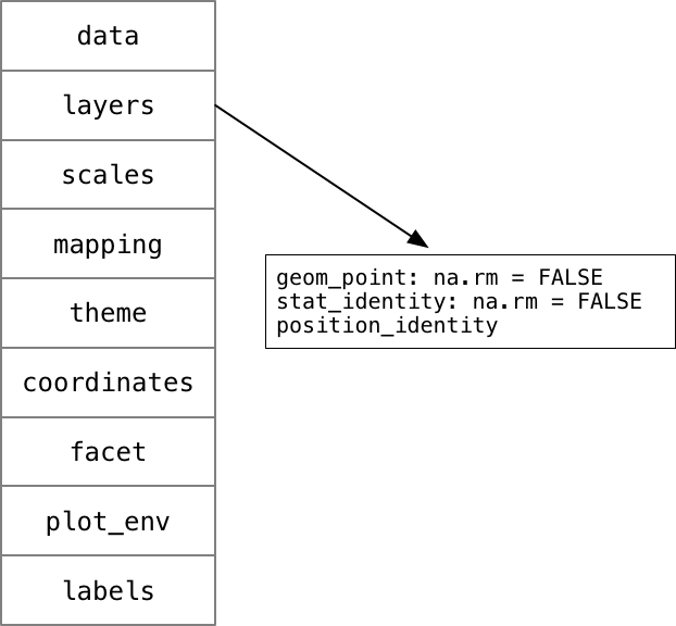
There is one layer with a Point Geom, an Identity Stat and an Identity Position. Make a mental note of that as it will become a familiar idiom if you get into the habit of making customized ggplot2 objects.
The scales element is a ScalesList object (see scales-.r in the ggplot2 source) which would contain scales you manually added to the ggplot object. Since the gg object is based on the minimal, seminal example, the defaults haven’t been computed yet (that’s ggplot_build(), coming up soon) so the length is 0 which can be verified with:
## [1] 0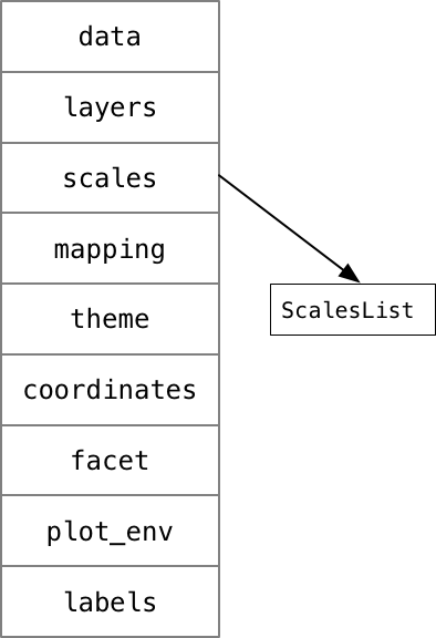
The mapping contains the aesthetic mappings that were created by one or more of the aes() family of functions. x, y and colour (note the spelling of that last one) all map to the expected data frame columns:
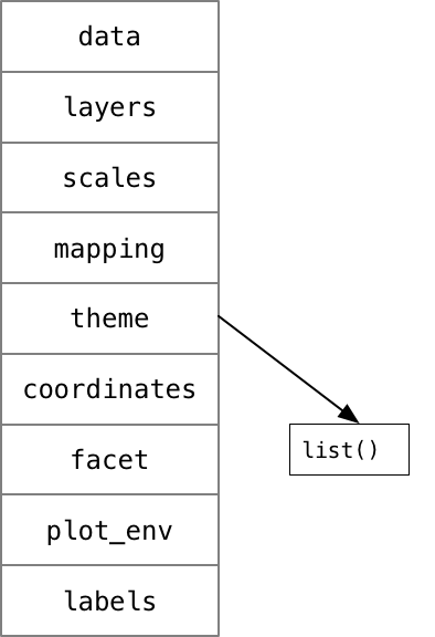
The theme element is also empty since an explicit theme has not been specified. When a theme is specified, the list structure will contain the details of all the various theme element settings (can can become quite long).
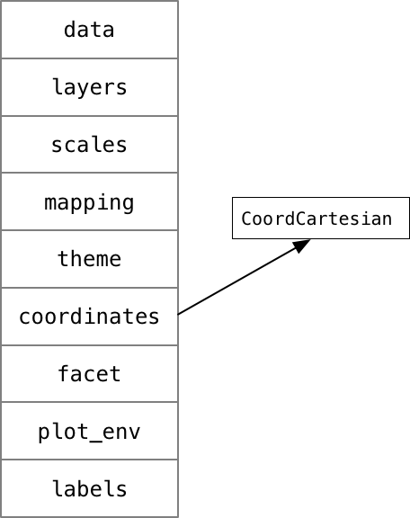
Unlike some of the other unspecified elements, the coordinates element does have a default value of CoordCartesian object:
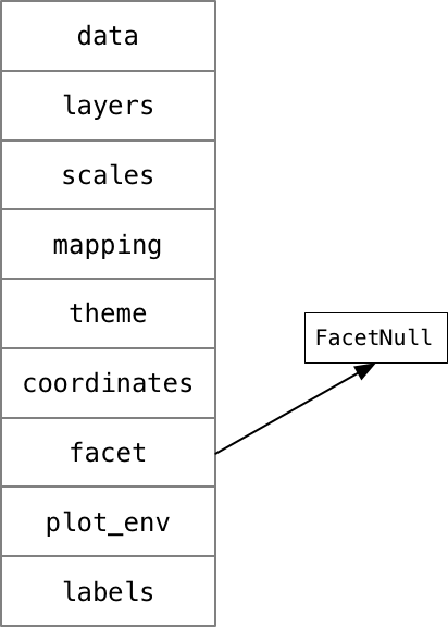
Since no faceting was specified, the default “null” facet is added to the plot in the facet element:
Penultimately, ggplot2 stores the environemnt where it will pick up plot values from (in this case, the global environemnt):
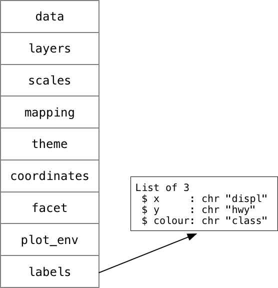
And, finally, ggplot2 shows off how smart it is by providing a list of the labels it managed to figure out from the mapped aesthetics:
Believe it or not — after all that — you’re really not much closer to having a visualization in front of you. A large chunk of the real work happens in ggplot_build().
1.3 The ggplot_built object
To examine a ggplot_buit object, it first needs to be created:
str(gb)
## List of 3
##  $ data  :List of 1
##  $ layout:Classes 'Layout', 'ggproto', 'gg' <ggproto object: Class Layout, gg>
##  $ plot  :List of 9
##   ..- attr(*, "class")= chr [1:2] "gg" "ggplot"
##  - attr(*, "class")= chr "ggplot_built"
Astute readers who are typing along at home will notice that the display is more compact than the actual str() since you’ve seen a number of the structures already in the previous verbose display. There are key differences that will be covered.
First up is the plot element. This contains a copy of data from the gg object itself but a few of the missing pieces have been filled in. In particular, the gb$plot$scales now has three Scale objects:
<ScaleContinuousPosition><ScaleContinuousPosition><ggproto object: Class ScaleDiscrete, Scale, gg>
which align with the x, y and colour column values that were passed in.
Now, the gb$plot$data element is still there and is the same as the gg$data element. However, there’s a new data element at the top level of gb and it’s a list, which suggests that it could — in other situations — contain more than one element. In this case there is one element and it is a data frame, but it is noticeably different than the one in gb$plot$data (NOTE: tibble::as_tibble() is being used to make the object display easier to read):
## # A tibble: 234 x 11
##    manufacturer      model displ  year   cyl      trans   drv   cty   hwy
##           <chr>      <chr> <dbl> <int> <int>      <chr> <chr> <int> <int>
##  1         audi         a4   1.8  1999     4   auto(l5)     f    18    29
##  2         audi         a4   1.8  1999     4 manual(m5)     f    21    29
##  3         audi         a4   2.0  2008     4 manual(m6)     f    20    31
##  4         audi         a4   2.0  2008     4   auto(av)     f    21    30
##  5         audi         a4   2.8  1999     6   auto(l5)     f    16    26
##  6         audi         a4   2.8  1999     6 manual(m5)     f    18    26
##  7         audi         a4   3.1  2008     6   auto(av)     f    18    27
##  8         audi a4 quattro   1.8  1999     4 manual(m5)     4    18    26
##  9         audi a4 quattro   1.8  1999     4   auto(l5)     4    16    25
## 10         audi a4 quattro   2.0  2008     4 manual(m6)     4    20    28
## # ... with 224 more rows, and 2 more variables: fl <chr>, class <chr>## # A tibble: 234 x 10
## colour x y PANEL group shape size fill alpha stroke
## <chr> <dbl> <dbl> <fctr> <int> <dbl> <dbl> <lgl> <lgl> <dbl>
## 1 #C49A00 1.8 29 1 2 19 1.5 NA NA 0.5
## 2 #C49A00 1.8 29 1 2 19 1.5 NA NA 0.5
## 3 #C49A00 2.0 31 1 2 19 1.5 NA NA 0.5
## 4 #C49A00 2.0 30 1 2 19 1.5 NA NA 0.5
## 5 #C49A00 2.8 26 1 2 19 1.5 NA NA 0.5
## 6 #C49A00 2.8 26 1 2 19 1.5 NA NA 0.5
## 7 #C49A00 3.1 27 1 2 19 1.5 NA NA 0.5
## 8 #C49A00 1.8 26 1 2 19 1.5 NA NA 0.5
## 9 #C49A00 1.8 25 1 2 19 1.5 NA NA 0.5
## 10 #C49A00 2.0 28 1 2 19 1.5 NA NA 0.5
## # ... with 224 more rowsThe original data has been transformed:
- there is a new, computed
colourcolumn that contains hex colors generated from the default discrete color scale (hue) - the original column names mapped to
xandyare now justxandy - there is a new
PANELcolumn which indicates which facet the associated data elements are to be drawn on (only one for this plot given the lack of facets) - a
groupcolumn has been added and computed based on the number of unique, discrete elements inmpg$class shape,size,fill,alphaandstrokehave also been added and set with the defaults for the aesthetic maps and parameters for the specified layers.
Remember this structure. When you build ggplot2 custom Geoms (and other objects) one big part of that is creating this structure (or, these structures if more than one data frame is being mapped to various aesthetics and shapes).
The layout element of the gb object is just a more detailed/complete/computed version of what was passed in from the gg object (more detail will be provided on that once the underlying structure of Geoms, Stats, etc are covered).
If you just enter gb at a console prompt you will see a plot due the ggplot-classed plot list element. Despite some transformations and data additions the plot is not yet ready for display. That’s the job of ggplot_gtable().
1.4 The gtable object
The details of the gtable object will be reviewed in a later chapter, but you do need to know a bit more about the object, now, before moving on to making your first Geom/Stat.
## TableGrob (10 x 9) "layout": 18 grobs
##     z         cells       name                                         grob
## 1   0 ( 1-10, 1- 9) background               rect[plot.background..rect.89]
## 2   5 ( 5- 5, 3- 3)     spacer                               zeroGrob[NULL]
## 3   7 ( 6- 6, 3- 3)     axis-l           absoluteGrob[GRID.absoluteGrob.31]
## 4   3 ( 7- 7, 3- 3)     spacer                               zeroGrob[NULL]
## 5   6 ( 5- 5, 4- 4)     axis-t                               zeroGrob[NULL]
## 6   1 ( 6- 6, 4- 4)      panel                      gTree[panel-1.gTree.17]
## 7   9 ( 7- 7, 4- 4)     axis-b           absoluteGrob[GRID.absoluteGrob.24]
## 8   4 ( 5- 5, 5- 5)     spacer                               zeroGrob[NULL]
## 9   8 ( 6- 6, 5- 5)     axis-r                               zeroGrob[NULL]
## 10  2 ( 7- 7, 5- 5)     spacer                               zeroGrob[NULL]
## 11 10 ( 4- 4, 4- 4)     xlab-t                               zeroGrob[NULL]
## 12 11 ( 8- 8, 4- 4)     xlab-b titleGrob[axis.title.x.bottom..titleGrob.34]
## 13 12 ( 6- 6, 2- 2)     ylab-l   titleGrob[axis.title.y.left..titleGrob.37]
## 14 13 ( 6- 6, 6- 6)     ylab-r                               zeroGrob[NULL]
## 15 14 ( 6- 6, 8- 8)  guide-box                            gtable[guide-box]
## 16 15 ( 3- 3, 4- 4)   subtitle         zeroGrob[plot.subtitle..zeroGrob.86]
## 17 16 ( 2- 2, 4- 4)      title            zeroGrob[plot.title..zeroGrob.85]
## 18 17 ( 9- 9, 4- 4)    caption          zeroGrob[plot.caption..zeroGrob.87]
The final object in the journey from grammar of graphics to final visualization is a grid graphics gtable object which is a structured representation of grobs — graphical objects — that contains everything necessary for the grid graphics system to transfer your visualization intent to an R graphics device.
For now, the most important thing to notice is that each top-level grob has:
- a
zrendering order top,right,bottom,left position extents incells- a
name(which is very important as you’ll see later) - the
grobitself (which could be – and likely is – a table or list of othergrobs)
To prove this is the final step, just do:
1.5 Exercises
Before moving on, you should get cozy with the ggplot and ggplot_built structures. Cozy enough that you should be able to read the output of str on them from other ggplot2 creations and be able to read them without too much reliance on the ggplot2 source code (using the source code as a reference is totally okay, though since the important part is familiarity and not wrote memorization).
To that end, try the following exercises:
- Incrementally build upon the initial, tiny example at the beginning of this chapter, changing and adding aesthetics, geoms, coordinates, themes, etc and examine the
ggandgbstructures after each one. See how they morph and grow. Don’t skimp on this part! You will get a better understanding of what you’re manipulating if you see how the standard/traditionalggplot2operations work. - Create or find a complex
ggplot2example that incorporates multiple data sources and fine-grained customization to see just how complex these objects can get and where various transformations take place. - For each of the above, look at the created
gtableand note any top-level differences. That introspection will come in handy later. - For each reference to a
ggprotoobject in anystr()output you create, make a “map” of whichggplot2source code file it is in. This will be an invaluable guide for you as you continue on this gg-journey.