hrbrmstr’s Year In Review

# Throughout this document there will be commentary in, well, comments.
# The code is not nearly as concise as I would have liked it to be, but such is the way of things.
# Once it's up on GitHub, do not hesitate to as questions in issues or even submit PRs for views you create.
#
# IMPORTANT set "include_wordpress" above to "no" if you aren't a wordpress users (or remove those code chunks)
library(gh) # devtools::install_github("r-lib/gh")
library(stackr) # devtools::install_github("dgrtwo/stackr")
library(pressur) # devtools::install_github("hrbrmstr/pressur")
library(jericho) # devtools::install_github("hrbrmstr/jericho") # implies rJava requirement
# NOTE: you also need scales and DT but I almost never library() them anymore
# I'm fairly certain I got them all here.
library(ggalt)
library(stringi)
library(anytime)
library(igraph)
library(ggraph)
library(urltools)
library(lubridate)
library(hrbrthemes)
library(rprojroot)
library(ggbeeswarm)
library(tidyverse)
rt <- find_rstudio_root_file()StackOverflow
I answer questions on StackOverflow to:
- teach new R users how to fish
- help experienced R users with gnarly issues
- explore new “worlds” in R (I — scarily — know way more about genes than I really should thanks to this)
I kinda-sorta knew where & how I spend my time there, but finally decided to help quanitify it a bit.
# You'll see this pattern quite a bit in this document, so I'll explain it here.
#
# API requests eat up your own API quota bits and also consume bandwidth and CPU
# time for the (free) services we all use. It's not cool to repeatedly hit the
# servers for data that doesn't change.
#
# Now, I'm not giving you my data, but this pattern will make it easier for you
# to cache your own results.
#
# A data file (RDS) is defined and checked for.
# If it does not exist, API calls are made and then cached into it
# If it does exist, the data is read from the cache.
#
# If you ever need to refresh the data, just [re]move the cached RDS files.
#
# The .gitignore _should_ keep your data off github, but you're responsible for
# that in the long run.

so_data_file <- file.path(rt, "data", "my_so.rds") # Where we're going to store cached SO data

if (!file.exists(so_data_file)) {

  # grab my answers for 2 years
  my_answers <- stack_users(
    params$stack_user, "answers",
    fromdate=as.integer(as.POSIXct(as.Date(sprintf("%s-01-01",
                                                   params$curr_year-1)))),
    todate=as.integer(as.POSIXct(as.Date(sprintf("%s-12-31", params$curr_year)))),
    pagesize=100,
    num_pages=50
  )

  # now get the question data for those answers (this was much easier on the SO data site with SQL btw)
  starts <- seq(1, length(my_answers$question_id), 100)
  ends <- c(starts[-1]-1, length(my_answers$question_id))

  map2_df(starts, ends, ~{
    stack_questions(my_answers$question_id[.x:.y], pagesize=100)
  }) -> my_answers_qs

  # grab my comments (I didn't rly do anything with them for the review)
  my_comments <- stack_users(
    params$stack_user, "comments",
    fromdate=as.integer(as.POSIXct(as.Date(sprintf("%s-01-01",
                                                   params$curr_year-1)))),
    todate=as.integer(as.POSIXct(as.Date(sprintf("%s-12-31", params$curr_year)))),
    pagesize=100,
    num_pages=50
  )

  # grab badge data for previous year (it doesn't come with the date so we have to do it this way)
  stack_users(
    params$stack_user, "badges",
    fromdate=as.integer(as.POSIXct(as.Date(sprintf("%s-01-01", params$curr_year-1)))),
    todate=as.integer(as.POSIXct(as.Date(sprintf("%s-12-31", params$curr_year-1)))),
    pagesize=100,
    num_pages=30
  ) %>%
    mutate(year = params$curr_year-1) -> my_badges_prev_year

  # and this year
  stack_users(
    params$stack_user, "badges",
    fromdate=as.integer(as.POSIXct(as.Date(sprintf("%s-01-01", params$curr_year)))),
    todate=as.integer(as.POSIXct(as.Date(sprintf("%s-12-31", params$curr_year)))),
    pagesize=100,
    num_pages=30
  ) %>%
    mutate(year = params$curr_year) -> my_badges_curr_year

  # finally, get my reputation
  my_rep <- stack_users(
    params$stack_user, "reputation-history",
    pagesize=100,
    num_pages=100
  )

  # bundle it up in a list (I regret not doing that for the other sections)
  list(
    my_answers = my_answers,
    my_answers_qs = my_answers_qs,
    my_comments = my_comments,
    my_badges = bind_rows(my_badges_prev_year, my_badges_curr_year),
    my_rep = my_rep
  ) -> my_so

  write_rds(my_so, so_data_file)
} else {
  my_so <- read_rds(so_data_file)
}

# clean up the answers and get it out of the list
tbl_df(my_so$my_answers) %>%
  mutate(month = as.Date(format(creation_date, "%Y-%m-01")),
         year = factor(lubridate::year(creation_date))) -> answers
I’m IRL “busier” these days and the waffle chart does reflect that I’ve not helped as many folks on SO this year (with new answers) as I did the previous one. However, the reduced answer count is also indicative of a deliberate shift into answering certain tags in preparation for writing another tome (which is reflected in the treemap to be presented in a bit).
# I got lucky here and didn't have to deal with an unven break due to the # of answers
# this bit may require tweaking if the same is not true for anyone else who runs the code.
count(answers, year) %>%
  mutate(year = sprintf("%s: %s (%s)", year,
                        scales::comma(n), scales::percent(n/sum(n)))) -> answers_wfl

waffle::waffle(answers_wfl, colors=c("lightslategray", "springgreen")) +
  labs(title="Answers Counts Across Years",
       subtitle=sprintf("%s answers between the past 2 years",
                        scales::comma(sum(answers_wfl$n)))) +
  theme_ipsum_rc(grid="") +
  theme(axis.text=element_blank()) +
  theme(legend.direction = "vertical") +
  theme(legend.position="bottom")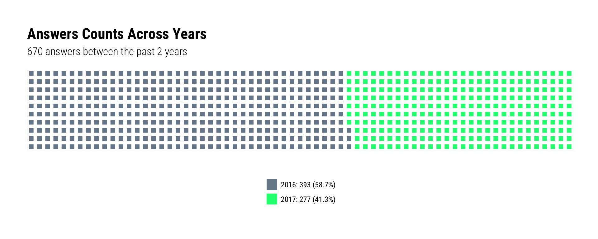
Despite being a bit more picky about which questions I answer, my answer acceptance rate hasn’t really improved. But, one reason for this in 2017 is that I made some efforts to go back in time on SO and add “modern R” answers to older questions, and the folks on SO who post questions have little incentive to go back to old questions for any reason (if David or Julia are reading this, it might be worth poking at a new badge or rep increase endorphin stimulus for question owners for this particular condition).
# this is quite a bit of work for just an annotated slope graph
count(answers, year, is_accepted) %>%
  mutate(is_accepted = ifelse(is_accepted, "Accepted", "Not Accepted")) %>%
  spread(year, n) -> answers_sg

prev_year <- as.character(params$curr_year-1)
curr_year <- as.character(params$curr_year)

gather(answers_sg, year, value, -is_accepted) %>%
  mutate(hjust = ifelse(year == prev_year, 1, 0)) %>%
  mutate(lab = ifelse(year == curr_year,
                      sprintf("%s %s", scales::comma(value), is_accepted),
                      scales::comma(value))) -> answers_sg_lab

gather(answers_sg, year, value, -is_accepted) %>%
  group_by(year) %>%
  mutate(pct = value/sum(value)) %>%
  filter(is_accepted == "Accepted") %>%
  mutate(pct = sprintf("%s Acceptance Rate: %s",
                       year, scales::percent(pct))) %>%
  pull(pct) %>%
  paste0(collapse="\n") %>%
  sprintf("%s\n", .) -> acceptance_rate

ggplot(answers_sg, aes(x=prev_year, xend=curr_year, color=is_accepted)) +
  geom_segment(aes_(y=as.name(prev_year),
                    yend=as.name(curr_year))) +
  geom_text(data=answers_sg_lab, family=font_rc,
            aes(x=year, y=value, hjust=hjust, label=lab),
            nudge_x=c(-0.01, -0.01, 0.01, 0.01)) +
  geom_text(data=data.frame(), aes(x=1.5, y=-Inf, label=acceptance_rate),
            color="#2b2b2b", vjust=0, lineheight=0.9, family=font_rc) +
  scale_x_discrete(expand=c(0,0.33), position = "top") +
  scale_color_manual(values=c("lightslategray", "slateblue"), guide=FALSE) +
  labs(x=NULL, y=NULL, title="Answer Acceptance Across Years", subtitle="") +
  theme_ipsum_rc(grid="X", axis_text_size = 14) +
  theme(legend.position="none") +
  theme(axis.text.y=element_blank())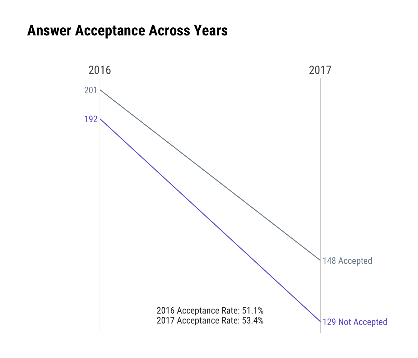
As noted, I’ve had quite a bit going on this year, which impacted the cadence from the previous year. One reason for more fall/winter activity in-general is that it helps combat seasonal affective disorder.
# 2018 will see me use xspline area charts since it mimics the smooth interpolated D3 charts
# without having to deal with widgets. I also don't use ggalt enough.
count(answers, year, month) %>%
  ggplot() +
  stat_xspline(geom="area", aes(month, n, fill=year, color=year),
               size=1, alpha=2/3) +
  scale_x_date(expand=c(0,0), date_labels="%b\n%Y") +
  scale_y_comma(expand=c(0,0), limits=c(0, 60)) +
  scale_color_manual(values=c("lightslategray", "springgreen"), guide=FALSE) +
  scale_fill_manual(values=c("lightslategray", "springgreen"), guide=FALSE) +
  facet_wrap(~year, ncol=2, scales="free_x") +
  labs(x=NULL, y="# Answers", title="Answers per Month") +
  theme_ipsum_rc(grid="XY") +
  theme(panel.spacing.x=unit(0, "null")) +
  theme(legend.position="none") +
  theme(axis.text.x=element_text(hjust=c(0, 0.5, 0.5, 0.5, 0.5)))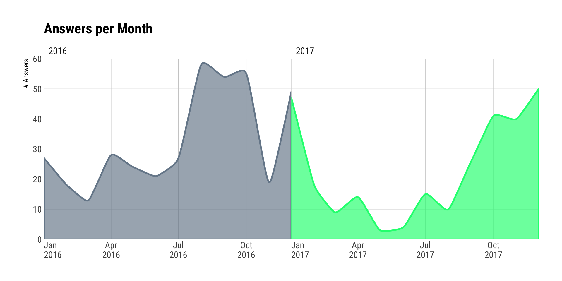
I was also curious about the questions associated with my top answers.
First a view of answer scores vs question views (this surprised me during EDA work, which is why I’m including it). One “SO FAIL” of mine is that I tend to gravitate towards pretty niche topics since they tend to be harder/more interesting (to me):
left_join(answers, my_so$my_answers_qs, "question_id") %>%
  filter(year==2017) %>%
  arrange(desc(view_count)) %>%
  select(score=score.x, title, tags, view_count, link) -> ans_score_q_view

# i love quasirandom charts. i probably use them too much, in fact. i also like to use this
# aesthetic pattern of slighly alpha on the fill with a white, thin stroke around the dot
# with a slightly larger dot.

ggplot(ans_score_q_view, aes(score, view_count)) +
  geom_quasirandom(fill="slateblue", color="white", size=3, stroke=0.5, shape=21, alpha=3/4) +
  scale_x_continuous(breaks=seq(min(ans_score_q_view$score), max(ans_score_q_view$score, 1))) +
  scale_y_continuous(label=scales::comma) +
  labs(x="Answer Score", y="# Question Views", title="Popularity of Questions by My Answer Scores") +
  theme_ipsum_rc(grid="XY")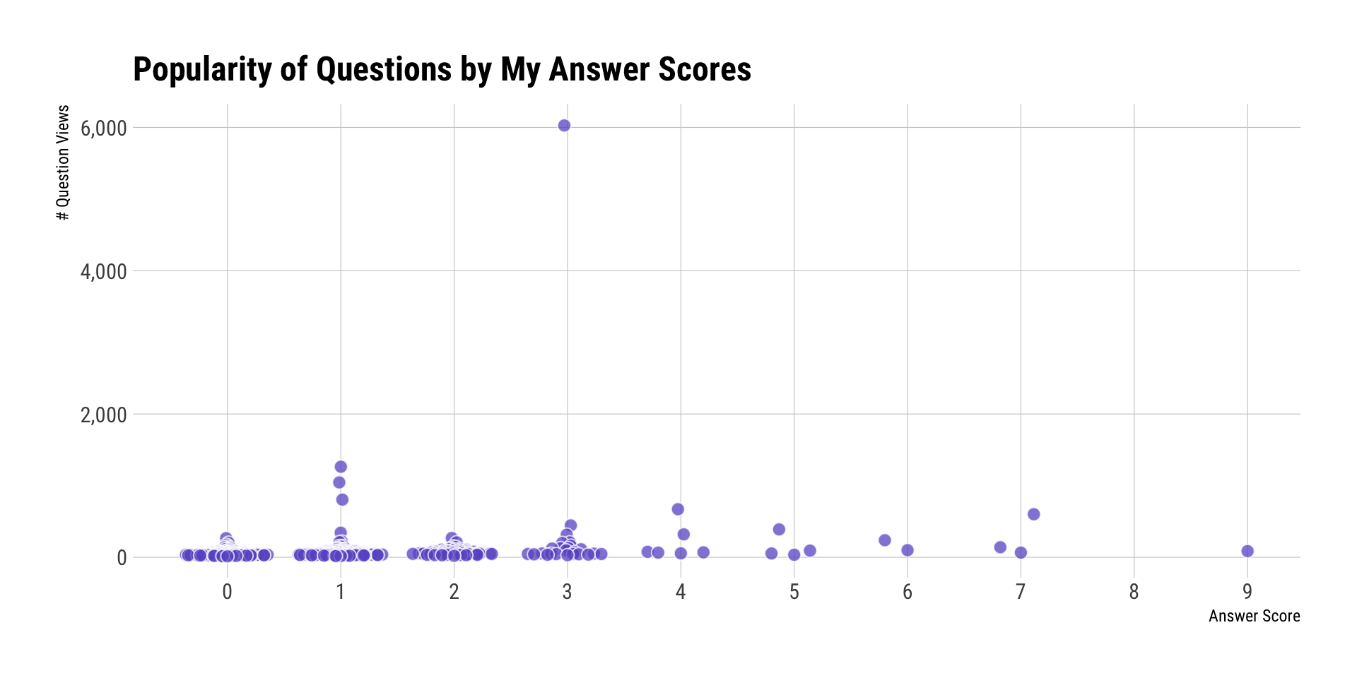
In case you were wondering that that 6,000+ question was, it was: Better way to convert list to vector?
These were my top 10 answers. Strangely enough, none of them were in the “web scraping” area of focus I had this year.
arrange(ans_score_q_view, desc(score)) %>%
  top_n(10, score) %>%
  DT::datatable(options = list(dom = 't')) # datatable makes things way too easy
The subtitle for the next graph says it all: What tags do I seem to gravitate towards answering and how has that changend in the last 24 months?. As noted, I’m not surprised by the focus on “web things” since it was deliberate. I can also correlate the reduced number of answers to no longer helping with gambling, sports or financial web scraping questions (for many reasons).
left_join(answers, my_so$my_answers_qs, "question_id") %>%
  select(year, tag=tags) %>%
  separate_rows(tag, sep=",") %>%
  count(year, tag) %>%
  mutate(year = as.character(year)) %>%
  mutate(year_tag = sprintf("%s-%s", year, tag)) -> year_tag_ct

# the rest is all setup for ggraph. We need to have it be "flare"-like and this
# is the shortest way I've found to do that. I'm definitely open to other
# suggestions and/or examples.

bind_rows(
  data_frame(name="", short_name="", year=NA, value=0),
  data_frame(name=unique(year_tag_ct$year), short_name=name,
             year=unique(year_tag_ct$year), value=0)
) %>%
  bind_rows(
    select(year_tag_ct, name=year_tag, short_name=tag, year=year, value=n)
  ) %>%
  mutate(short_name = ifelse(value > 1, short_name, "")) -> verts

bind_rows(
  data_frame(from=c(""), to=unique(as.character(year_tag_ct$year))),
  select(year_tag_ct, from=year, to=year_tag)
) -> tag_graph_df

g <- graph_from_data_frame(tag_graph_df, vertices = verts)

ggraph(g, "treemap", weight="value") +
  geom_node_tile(aes(fill = year), size = 0.25) +
  ggraph::geom_node_text(aes(label=stri_replace_all_fixed(short_name, "-", "\n"),
                             size=value), lineheight=0.9, color="white", family=font_rc) +
  scale_size_continuous(range=c(2, 10), guide = FALSE) +
  scale_fill_manual(name=NULL,
                    values=c("lightslategray","slateblue"),
                    breaks=c(curr_year, prev_year)) +
  labs(x=NULL, y=NULL, title="SO Question Annual Tag Gravity",
       subtitle="What tags do I seem to gravitate towards answering and how has that changend in the last 24 months?") +
  theme_ipsum_rc(grid="") +
  theme(axis.text=element_blank())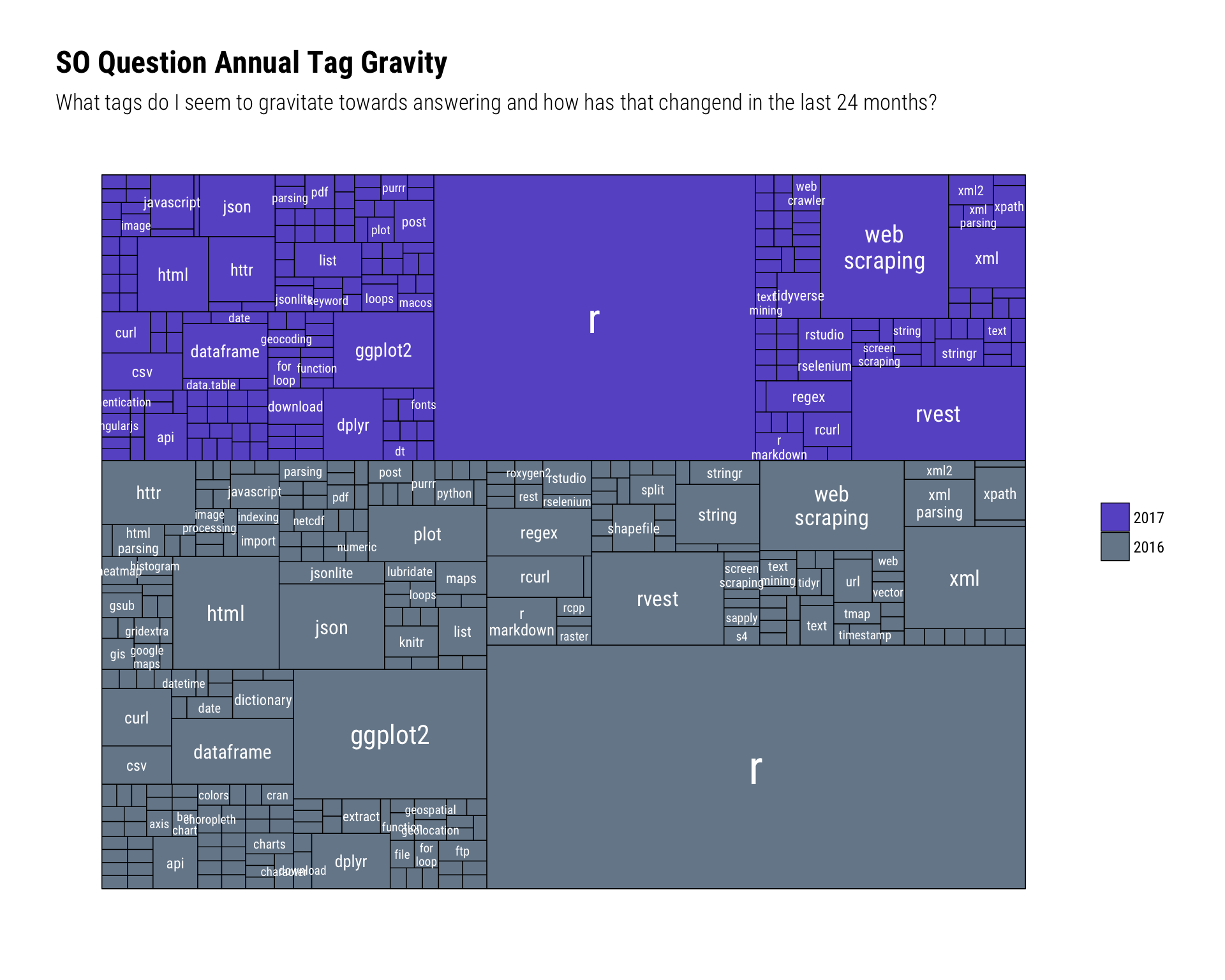
The “reputation trend” chart is a pretty boring visualization and I almost didn’t include it, but wanted to see if there were any surprises in the reputation cadence. An artefact of being on SO for a long time is that one’s older answers help prop up reputation even if one’s current activity has waned a bit.
tbl_df(my_so$my_rep) %>%
  mutate(month = as.Date(format(creation_date, "%Y-%m-01")),
         year = lubridate::year(creation_date)) -> rep

count(rep, year, month, wt=reputation_change) %>%
  mutate(cumsum = cumsum(n)) %>%
  filter(year>=params$curr_year-1) %>%
  ggplot() +
  stat_xspline(geom="area", aes(month, cumsum),
               color="slateblue", fill="slateblue", size=1, alpha=2/3) +
  scale_x_date(expand=c(0,0), date_labels="%b\n%Y") +
  scale_y_comma(expand=c(0,0)) +
  labs(x=NULL, y="# Answers", title="Reputation Trend") +
  theme_ipsum_rc(grid="XY") +
  theme(panel.spacing.x=unit(0, "null")) +
  theme(legend.position="none")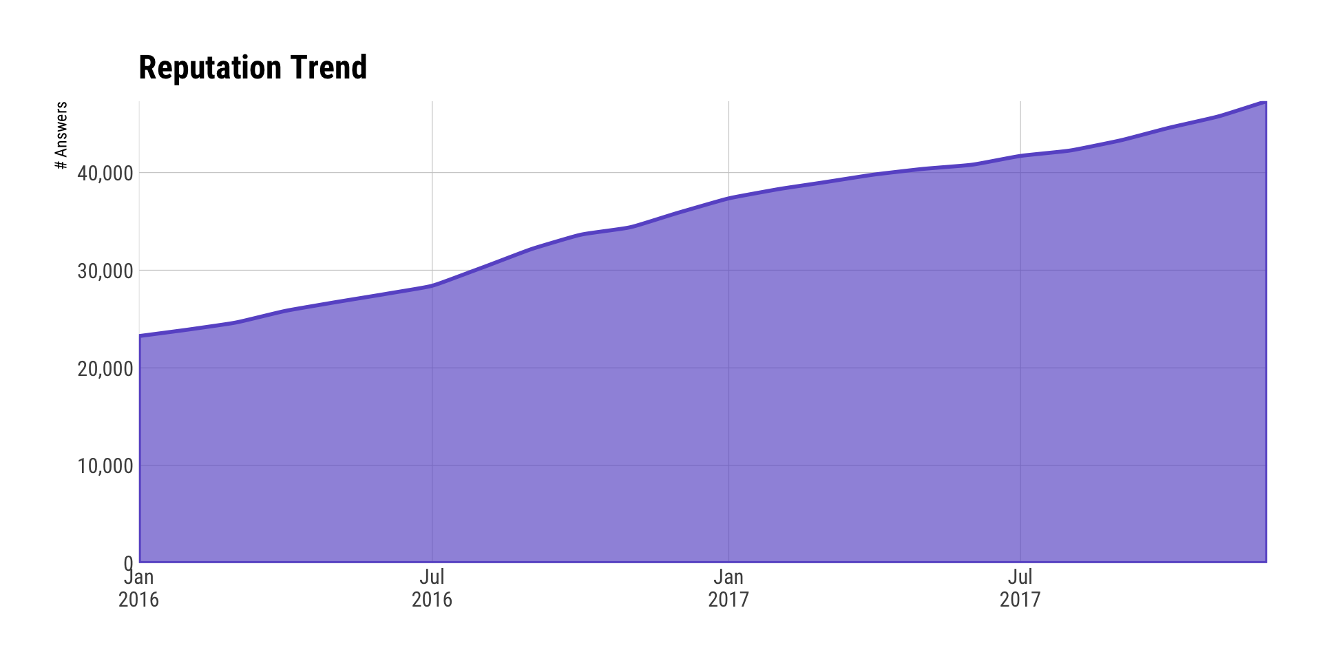
Despite initial appearances, this next vis isn’t just a humblebrag. I wanted to validate some (most) of my previous assertions about reputation gaining and I think this view does that — especially for “Necromancer” and “Nice Answer” — but, also the fact that badges can accumulate faster if older answers get upticks from new folks in search of answers.
# in retrospect, this is _alot_ of customization
tbl_df(my_so$my_badges) %>%
  count(badge_type, year, name, rank, wt=award_count, sort=TRUE) %>%
  mutate(name = factor(name, levels=rev(unique(name)))) %>%
  mutate(badge_type = stri_trans_totitle(stri_replace_first_fixed(badge_type, "_", " "))) -> badge_df

ggplot(badge_df, aes(n, name)) +
  geom_point(aes(size=n, color=rank, fill=rank), stroke=1, alpha=3/4) +
  scale_x_continuous(expand=c(0,1), breaks=c(1, 5, 10, 15, 20), limits=c(1, 20)) +
  scale_y_discrete(expand=c(0,1.25)) +
  scale_color_manual(name=NULL, values=c("#cd7f32", "#ffd700", "#c0c0c0")) + # TODO name these colors
  scale_fill_manual(name=NULL, values=c("#cd7f32", "#ffd700", "#c0c0c0")) +
  scale_size_area(name=NULL, max_size=10) +
  facet_grid(badge_type~year, scales="free_y", switch="y") +
  labs(x=NULL, y=NULL, title="Badges Earned by Type & Year") +
  theme_ipsum_rc(grid="XY") +
  theme(strip.placement="outside") +
  theme(strip.text.y=element_text(angle=360)) +
  theme(panel.spacing.y=unit(0, "null")) +
  theme(legend.box="horizontal") +
  theme(legend.direction="horizontal") +
  theme(legend.background=element_rect(fill="white", color="white")) +
  theme(legend.position=c(0.5, 0.475))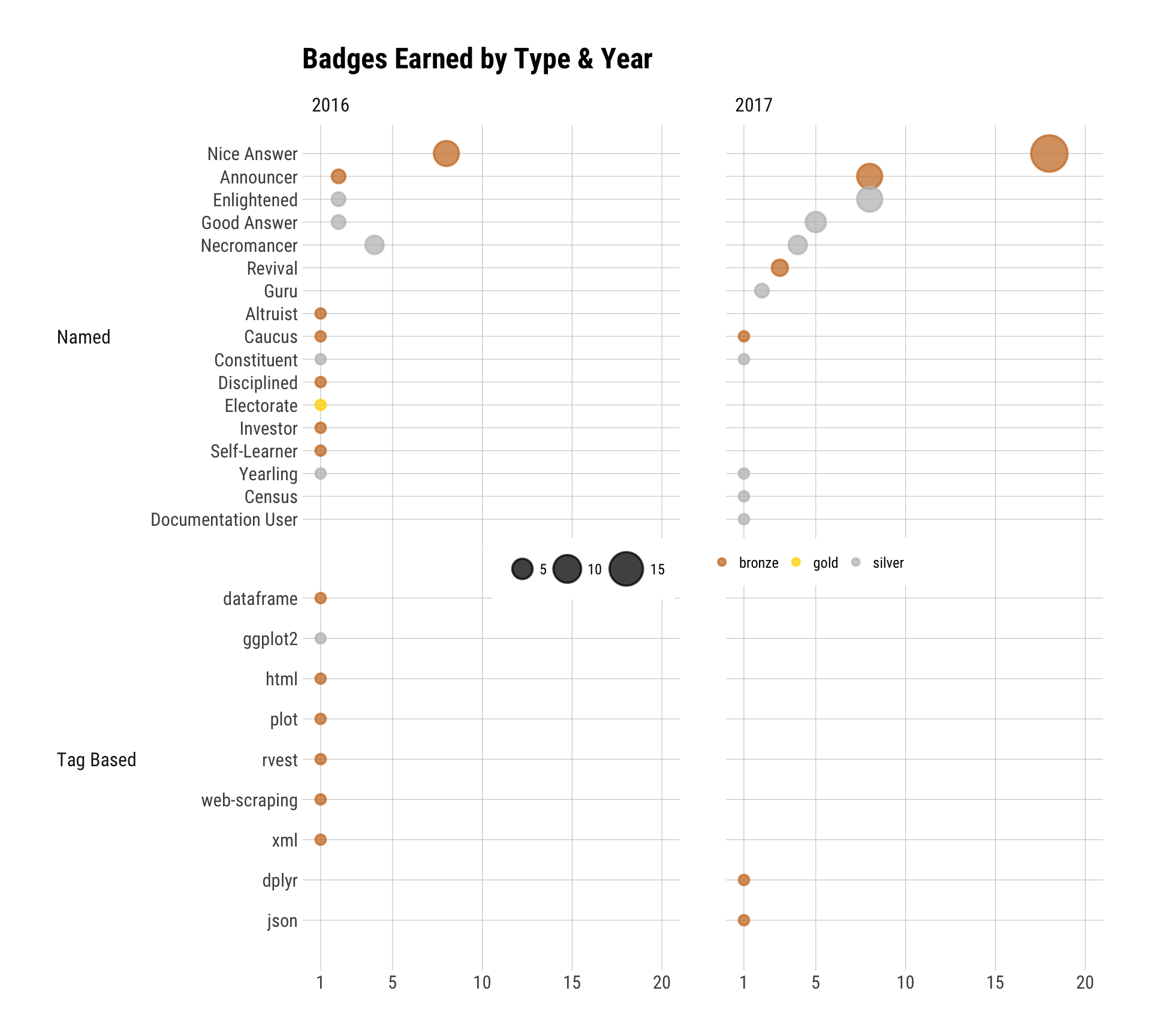
Reflection & Speculation
I continue to firmly believe you can truly significantly help others (I’ve had numerous folks tell me that an answer helped them through gnarly areas of thesis writing or work-problems) and hone+expand your own skills by answering questions on SO. While reputation counters and badges are nice, I’m not really “in it” for the bling, but more for said impact. A major pre-regret of 2018 is that I won’t have as much time in the first six months of the year due to book writing and teaching, but I also hope those activities result in helping as many if not more folks with R-centric data science questions.
GitHub
I’ll be up-front about not knowing what I wanted to track from GitHub. I’m not “graded” at work or at home on GH commits (well, I don’t think @mrshrbrmstr judges me by GH commits). As noted, I do what I do to help folks, not for the bling. I’m also a bit reticent to have stars, watches or forks indicate utility of something since many folks use such things for “bookmarks” (I know I do). I push stuff to GH primarily to supplement blogs or stage packages, and I’m not sure I’d change behaviour based on any data views, here, but shall endeavour to look at the data in ways not easily done via GH itself.
s_ghn <- safely(gh_next) # API calls are fraught with peril, so make this one a bit safer

my_repos_file <- file.path(rt, "data", "my_repos.rds")

if (!file.exists(my_repos_file)) {
  curr_repo <- gh("/user/repos", username = "public")
  my_repos <- list()
  i <- 1
  my_repos[i] <- list(curr_repo)
  spin <-  TRUE
  while(spin) {
    curr_repo <- s_ghn(curr_repo)
    if (is.null(curr_repo$result)) break
    i <- i + 1
    curr_repo <- curr_repo$result
    my_repos[i] <- list(curr_repo)
  }
  my_repos <- unlist(my_repos, recursive=FALSE)
  write_rds(my_repos, my_repos_file)
} else {
  my_repos <- read_rds(my_repos_file)
}

# only public repos, pls
public_repos <- keep(my_repos, ~.x$owner$login == params$gh_user & !.x$private)
public_repo_count <- length(public_repos)

map_df(public_repos, ~{
  data_frame(
    name = .x$name,
    created = anytime::anytime(.x$created_at),
    updated = anytime::anytime(.x$updated_at),
    stars = .x$stargazers_count,
    watchers = .x$watchers_count,
    lang = .x$language %||% NA_character_
  )
}) -> repo_meta
I’ll engage in the “two years” comparisons in a bit. but I’ve never really stopped to look at my “top” repos, so will start with some top 20 views.
mutate(repo_meta) %>%
  mutate(days_alive = ceiling(as.numeric(updated - created, "days"))) %>%
  top_n(20, wt=stars) %>%
  arrange(desc(stars)) -> top_20

# there's _alot_ of code here as I was going to do more with the data
# but really didn't care abt the punch card views at all after seeing them.
# i left the code in b/c i do use some of the data later on and others
# may want to poke at it more than i did.

my_punch_card_file <- file.path(rt, "data", "punch_cards.rds")

if (!file.exists(my_punch_card_file)) {
  pull(top_20, name) %>%
    map(~{
      gh("/repos/:owner/:repo/stats/punch_card", owner=params$gh_user, repo=.x)
    }) -> punch_cards
  write_rds(punch_cards, my_punch_card_file)
} else {
  punch_cards <- read_rds(my_punch_card_file)
}

n <- if (length(punch_cards) > 20) 20 else length(punch_cards)

map_df(1:n, ~{
  map_df(punch_cards[[.x]], ~set_names(.x, c("day", "hour", "Commits"))) %>%
    mutate(repo = top_20$name[.x])
}) %>%
  mutate(repo = factor(repo, levels=unique(repo))) -> punch_cards_df

my_repo_activity_file <- file.path(rt, "data", "repo_activity.rds")

if (!file.exists(my_repo_activity_file)) {
  pull(top_20, name) %>%
    map(~{
      gh("/repos/:owner/:repo/stats/commit_activity", owner=params$gh_user, repo=.x)
    }) -> repo_activity
  write_rds(repo_activity, my_repo_activity_file)
} else {
  repo_activity <- read_rds(my_repo_activity_file)
}

n <- if (length(repo_activity) > 20) 20 else length(repo_activity)

map_df(1:n, ~{
  map_df(repo_activity[[.x]], ~{
    .x$days <- set_names(.x$days, c("Sun", "Mon", "Tue", "Wed", "Thu", "Fri", "Sat"))
    flatten(.x)
  }) %>%
    mutate(repo = top_20$name[.x])
}) %>%
  mutate(week = anytime::anydate(week)) %>%
  mutate(repo = factor(repo, levels=unique(repo))) %>%
  select(-total) %>%
  gather(day, commits, -week, -repo) %>%
  mutate(day = factor(day, levels=c("Sun", "Mon", "Tue", "Wed", "Thu", "Fri", "Sat"))) -> repo_activity_df

wk_cnt_df <- count(repo_activity_df, repo, week, wt=commits)
For lack of knowledge of any other metric, I’m defining “top” by GitHub stars. To that end, the following shows the weekly commit activity (or, as I have dubbed it “commit pulse”) for my “top 20” repos in 2017:
# smooth area xspline and some facet strip hackery here. no magic.
ggplot(wk_cnt_df) +
  stat_xspline(geom="area", aes(week, n, group=repo), fill="slateblue", color="slateblue", size=0.5, alpha=2/5) +
  scale_x_date(expand=c(0,0), date_labels="%b\n%Y") +
  scale_y_continuous(expand=c(0,0), limits=c(0, max(wk_cnt_df$n)+2)) +
  facet_wrap(~repo, ncol=1, strip.position="left") +
  labs(x=NULL, y=NULL, title=sprintf("Top 20 Repos Commit Pulse by Week in %s", params$curr_year),
       subtitle=sprintf("Y-axis range is 0-%s (commits)",max(wk_cnt_df$n))) +
  theme_ipsum_rc(grid="X") +
  theme(panel.spacing.y=unit(-10, "pt")) + # tweak this if you want more vertical spacing
  theme(strip.text.y=element_text(angle=360, hjust=1, vjust=-1, size=10, family=font_rc)) +
  theme(axis.text.y=element_blank()) +
  theme(axis.text.x=element_text(hjust=c(0, rep(0.5, 3))))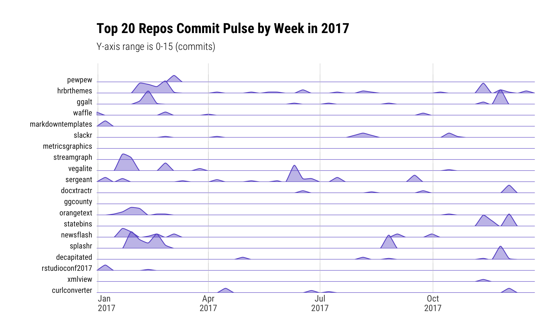
This tracks well with active memory. I deliberately spent quite a bit of time on hrbrthemes, sergeant, splashr and decapitated since they help me with daily work-work but also felt they’d be useful to the broader community.
The late-in-the-year bumps for some of the packages (most of the repos I have are R packages) was also a deliberate attempt to get some updates on CRAN before 2017 came to a close. Alas, most will have to wait for 2018 since I don’t like to bug CRAN with too many maintenance updates in a year and had ideas for improved functionality in most of them as I tidied them up.
I did have more activity in-general on GitHub this year when compared to the previous one:
mutate(
  repo_meta,
  year = lubridate::year(created),
  week = lubridate::week(created)
) %>%
  filter(year %in% c(params$curr_year-1, params$curr_year)) -> gh_two_years

count(gh_two_years, year) %>%
  mutate(lab = sprintf("%s: %s new repos", year, n)) %>%
  pull(lab) %>%
  paste0(collapse = "\n") -> rep_sub

count(gh_two_years, year, week) %>%
  mutate(date = as.Date(sprintf("%s-%02d-1", year, week), "%Y-%U-%u")) %>%
  mutate(year = factor(year)) %>% # I rly want to break this pipe but can't justify it
  ggplot(aes(date, n)) +
  geom_segment(aes(xend=date, yend=0, color=year), size=1) +
  scale_x_date(expand=c(0,15), date_label="%b\n%Y") +
  scale_y_continuous(breaks=seq(0, 10, 2), limits=c(0,10)) +
  scale_color_manual(values=c("lightslategray", "springgreen"), guide=FALSE) +
  scale_fill_manual(values=c("lightslategray", "springgreen"), guide=FALSE) +
  labs(x=NULL, y=NULL, title="New Repos per Week", subtitle=rep_sub) +
  theme_ipsum_rc(grid="Y") +
  theme(legend.position="none") +
  theme(panel.spacing.x=unit(0, "null"))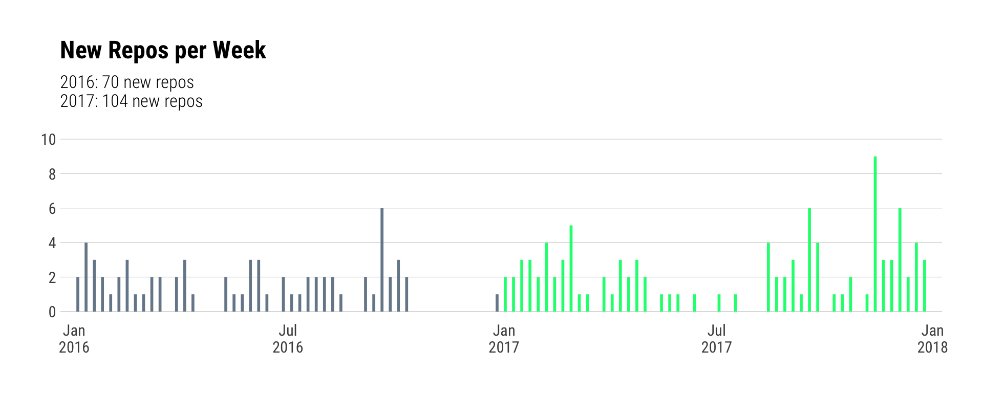
s_gh <- safely(gh) # empty repos will cause an error for the calls we're going to make

repo_pkgs_file <- file.path(rt, "data", "repo_pkgs.rds")

if (!file.exists(repo_pkgs_file)) {
  pull(gh_two_years, name) %>%
    map(~{
      s_gh("/repos/:owner/:repo/contents/:path", owner=params$gh_user, repo=.x, path="/")$result
    }) -> repo_pkgs
  write_rds(repo_pkgs, repo_pkgs_file)
} else {
  repo_pkgs <- read_rds(repo_pkgs_file)
}

map(repo_pkgs, ~map(.x, 'url')) %>%
  flatten() %>%
  flatten_chr() %>%
  keep(stri_detect_fixed, "DESCRIPTION") %>%
  stri_match_first_regex(sprintf("/(%s)/([[:alnum:]\\-\\_]+)/", params$gh_user)) %>%
  .[,3] %>%
  discard(is.na) -> are_packages

filter(gh_two_years, name %in% are_packages) %>%
  mutate(year = factor(year)) %>%
  mutate(lab=sprintf("%s (%s*)", name, scales::comma(stars))) -> pkgs
How many packages did I release (on GitHub) in 2017 vs 2016?
This first view was mostly for fun (it’s hard to read the individual names) but I can see most of the most “popular” pacakges over the past two years from it:
ggplot(pkgs, aes(created, stars, label=lab, color=year)) +
  geom_point(size=0.5) +
  geom_text(aes(size=stars), lineheight=0.9, vjust=1) +
  scale_x_datetime(expand=c(0.125, 0), date_breaks="3 months", date_labels="%b\n%Y") +
  scale_y_continuous(trans="sqrt") +
  scale_color_manual(name=NULL, values=c("lightslategray", "slateblue")) +
  scale_size_continuous(range=c(1.5,6)) +
  labs(x="Package Repo Creation Date", y="# GitHub Stars",
       title="Package Creation and 'Popularity' : Take 1 (discrete package view)",
       subtitle="NOTE: Y-axis sqrt scale") +
  theme_ipsum_rc(grid="XY") +
  theme(legend.position="none")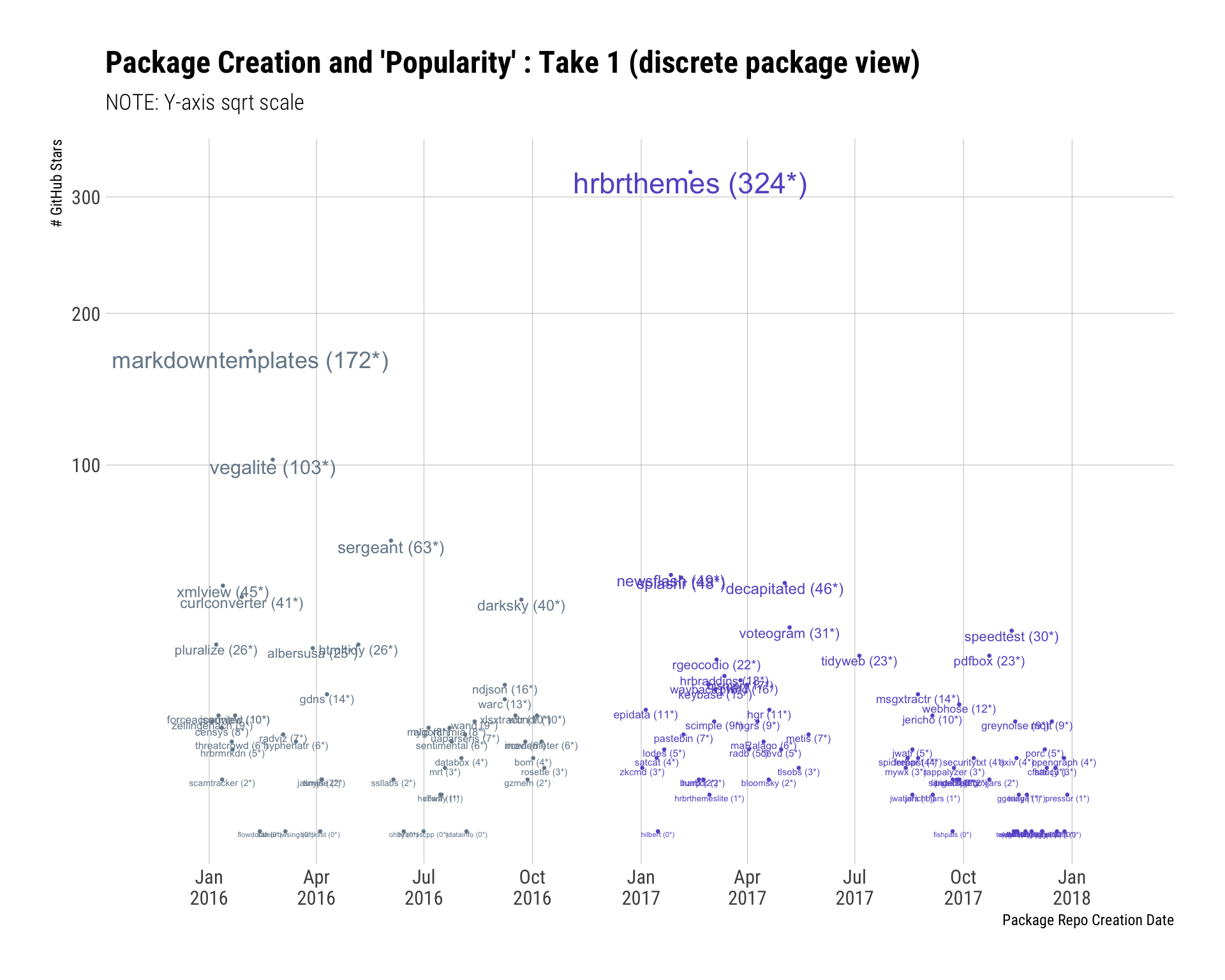
count(pkgs, year) %>%
  mutate(lab = sprintf("%s\n(%s packages released)", year, scales::comma(n))) %>%
  pull(lab) -> yr_lab

ggplot(pkgs, aes(year, stars)) +
  geom_quasirandom(aes(fill=year), width=0.25, size=3, color="white", stroke=0.5, alpha=3/4, shape=21) +
  scale_x_discrete(labels=yr_lab) +
  scale_fill_manual(name=NULL, values=c("lightslategray", "slateblue")) +
  labs(x=NULL, y="# GiHub Stars", title="Package Creation and 'Popularity' : Take 2 (annual summary view)") +
  theme_ipsum_rc(grid="XY") +
  theme(legend.position="none")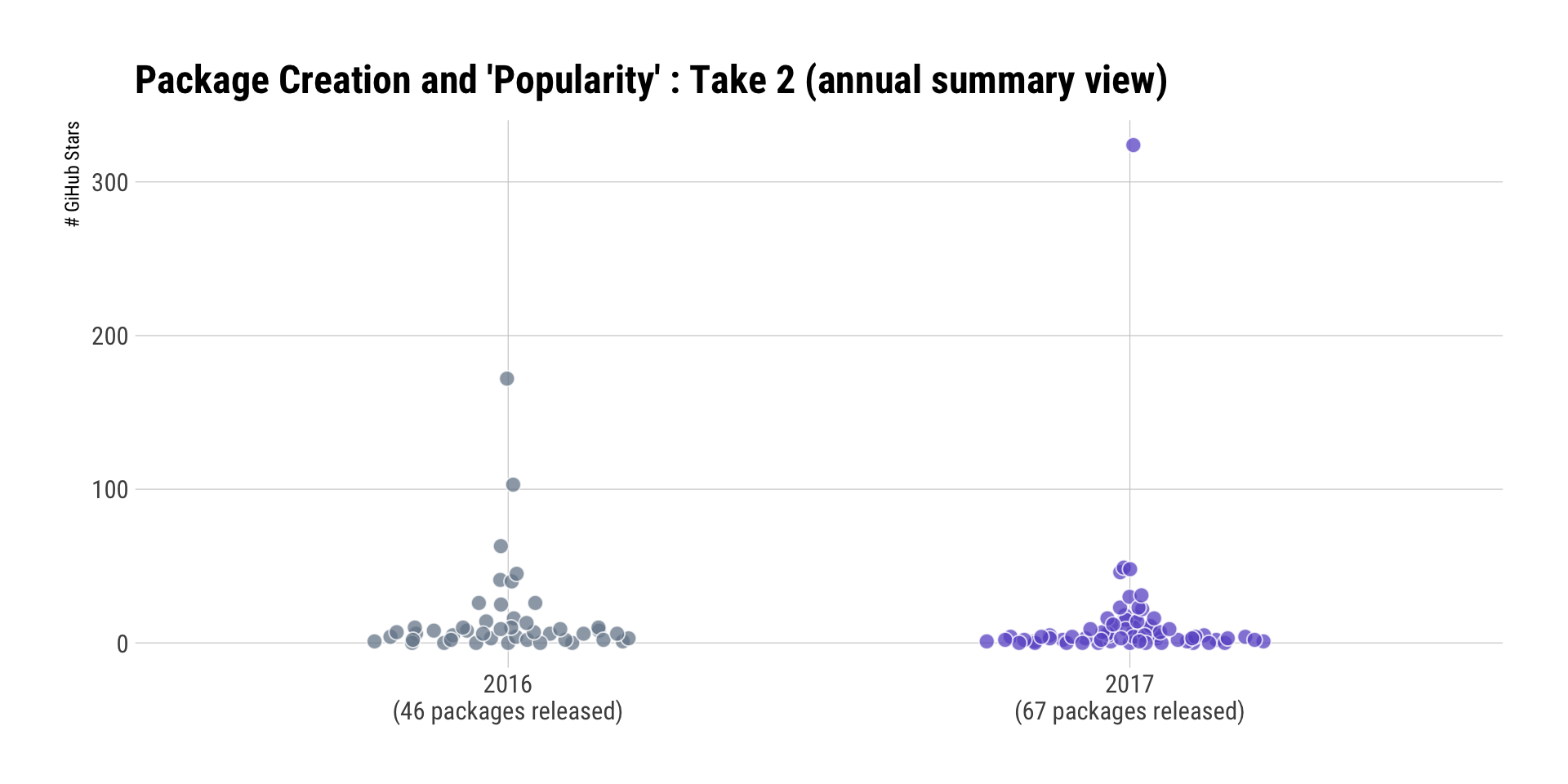
Reflection & Speculation
The increase in the number of packages is due, in-part, to my tendency towards SODD. However, I also make a package when I need some functionality but refuse to use source() since I’m adamant that such practices are — in the long run — unsustainable. And, if I need something it’s highly likely at least one other human will need it, and that’s a good enough reason to formalize the functionality into a package.
Having said that, package maintenance has become an emerging issue for me as users of slackr will be glad to point out. Not all of these GitHub-homed packages are on CRAN, but more than a few are. I started “cleaning house” in Q4 and have archived a few repos and consolidated functionality of some into other packages. I’m going to be very picky about what I put on CRAN moving forward, but will also be releasing a slew of new ones to CRAN in support of the forthcoming web scraping tome. There will be a drat repo setup for it, but they need to be on CRAN too so “devtools” is not a barrier to entry for readers.
I also need to start using PR and Issue templates and figure out a way to make it easier for folks to contribute.
Blogging
# YOU NEED to open up the project and execute this line BEFORE you run the RMD
# if you're including WordPress. If you're not including wordpress set the YAML
# parameter to "no".
#
# the .gitignore won't cache your oauth tokens on github.
#
# this line has to run in-Rmd at least once to prime the data cache.
wp_auth()

wp_user_file <- file.path(rt, "data", "wp_me.rds")
wp_posts_file <- file.path(rt, "data", "wp_posts.rds")
if (!file.exists(wp_user_file)) {
  me <- wp_about_me()
  write_rds(me, wp_user_file)
  my_posts <- wp_get_my_posts()
  write_rds(my_posts, wp_posts_file)
} else {
  me <- read_rds(wp_user_file)
  my_posts <- read_rds(wp_posts_file)
}

# for the record: it was slightly cumbersome retrofitting the Rmd to
# take a year as parameter. but i hope it's worth it for next year.
wp_two_years <- filter(my_posts, lubridate::year(date) %in% c(params$curr_year-1, params$curr_year))

wp_two_years_file <- file.path(rt, "data", "wp_two_years.rds")
if (!file.exists(wp_two_years_file)) {
  pb <- progress_estimated(nrow(wp_two_years))
  mutate(wp_two_years, post_stats = map(post_id, ~{
    pb$tick()$print()
    wp_post_stats(me$primary_blog, .x)
  })) %>%
    mutate(content_char = map_chr(content, jericho::html_to_text)) %>%
    mutate(word_count = stri_count_words(content_char)) %>%
    mutate(char_count = nchar(content_char)) -> wp_two_years
  write_rds(wp_two_years, wp_two_years_file)
} else {
  wp_two_years <- read_rds(wp_two_years_file)
}

left_join(
  map2_df(wp_two_years$post_id, wp_two_years$post_stats, ~{
    list(
      post_id = c(.x, .x),
      year = c(params$curr_year-1, params$curr_year),
      total = c(.y$years[[1]][[as.character(params$curr_year-1)]]$total %||% 0,
                .y$years[[1]][[as.character(params$curr_year)]]$total %||% 0)
    )
  }),
  select(wp_two_years, post_id, date, word_count, char_count),
  by="post_id"
) %>%
  mutate(year_created = lubridate::year(date)) %>%
  select(-date) -> totals

group_by(totals, year_created) %>%
  filter(year==year_created) %>%
  summarise(
    posts = n(),
    post_count_summary = list(broom::tidy(summary(total))),
    word_stats_summary = list(broom::tidy(summary(word_count))),
    char_stats_summary = list(broom::tidy(summary(char_count)))
  ) -> year_summary

# it feels like I shld have done this in a more tidy way

bind_rows(
  unnest(year_summary, word_stats_summary) %>%
    select(-post_count_summary, -char_stats_summary) %>%
    mutate(measure = "Post Word Count")
  ,
  unnest(year_summary, char_stats_summary) %>%
    select(-post_count_summary, -word_stats_summary) %>%
    mutate(measure = "Post Character Count")
  ,
  unnest(year_summary, post_count_summary) %>%
    select(-char_stats_summary, -word_stats_summary) %>%
    mutate(measure = "Post Views")
) %>%
  mutate(year_created = factor(year_created)) %>%
  mutate(measure = factor(measure,
                          levels=c("Post Character Count", "Post Word Count",
                                   "Post Views"))) -> post_dist
I ended up writing a new package pressur for this section as I wanted clean/quick access to blog stats and I use WordPress for blogging. As noted more than once, I’m in cybersecurity and have had to help many folks with WordPress security issues over the years and the only way to continue to be able to do that is to run it. I also have a teensy bit of honeypot code in the one I run so I can see attacker behaviour. WordPress counts things well and it saves me from relying on Google or having to save my access logs for too long.
Beyond some in-week stats reviews, I haven’t looked at WP stats in any real way before and I had some questions I wanted answered:
- Has my blathering changed in the past two years (i.e. post frequency and post attributes)
- What were my top posts in 2017
I have been eeriely consistent across the past two years in terms of how much I blather per-post. I remember going dark during the election and it further shows here.
mutate(wp_two_years, year = factor(lubridate::year(date))) %>%
  mutate(month = as.Date(format(date, "%Y-%m-01"))) %>%
  count(year, month) -> posts_year_month

count(posts_year_month, year, wt=n) %>%
  mutate(lab=sprintf("# Posts in %s: %s", year, nn)) %>%
  pull(lab) %>%
  paste0(collapse="\n") -> post_year_sum # this block alone is one big reason I try not to pipe into ggplot2

ggplot(posts_year_month, aes(month, n, color=year)) +
  geom_segment(aes(xend=month, yend=0), size=2) +
  scale_x_date(date_breaks="3 months", date_labels="%b\n%Y") +
  scale_color_manual(name=NULL, values=c("lightslategray", "springgreen"), guide=FALSE) +
  labs(x=NULL, y="# Posts", title="Posts Published per Month", subtitle=post_year_sum) +
  theme_ipsum_rc(grid="Y")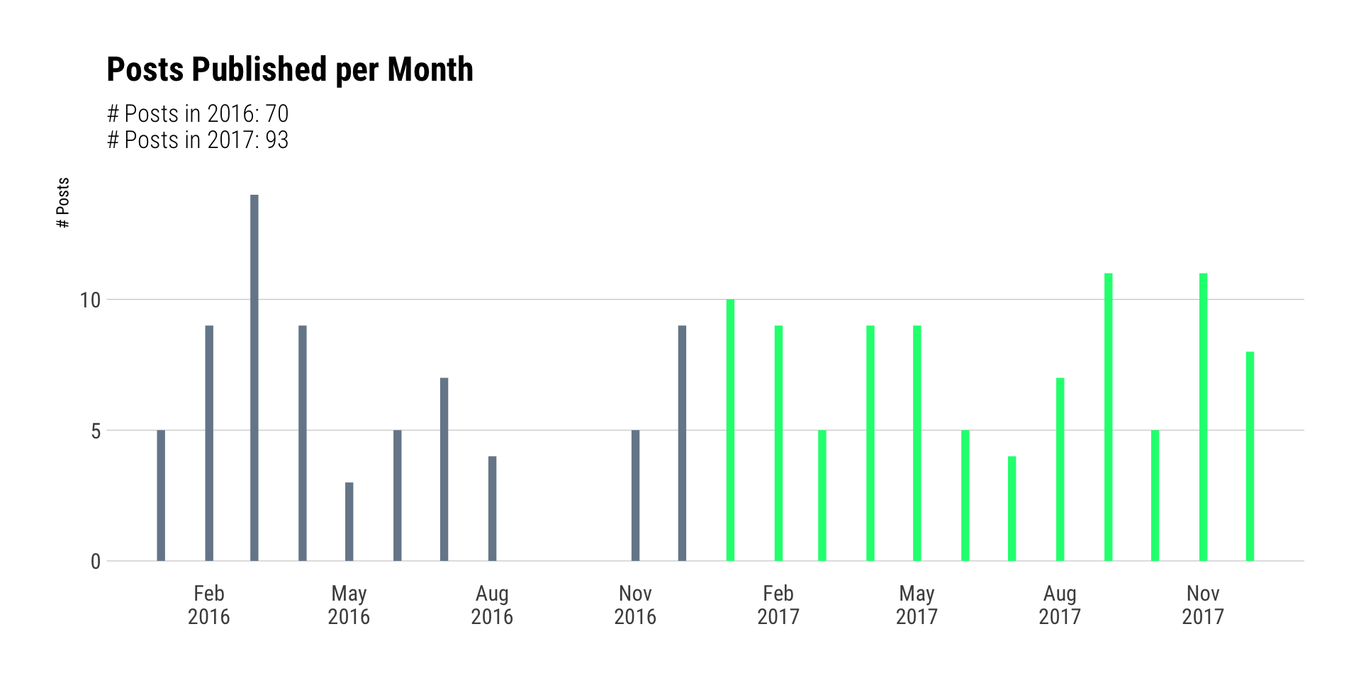
WannaCry helped boost interest in the bitcoin-related post which severely skewed the “Views”.
# yeah, yeah. boxplots. i know.
ggplot(post_dist) +
  geom_boxplot(aes(year_created, lower=q1, upper=q3, middle=median, ymin=minimum,
                   ymax=maximum, group=measure, fill=year_created), stat="identity") +
  scale_y_comma() +
  scale_fill_manual(name=NULL, values=c("lightslategray", "springgreen"), guide=FALSE) +
  facet_wrap(~measure, scales="free") +
  labs(x=NULL, y=NULL, title="Blog Post Meta Stats (selected distributions)",
       subtitle="NOTE Free Y scales; Character/word count does not include source code") +
  theme_ipsum_rc(grid="Y")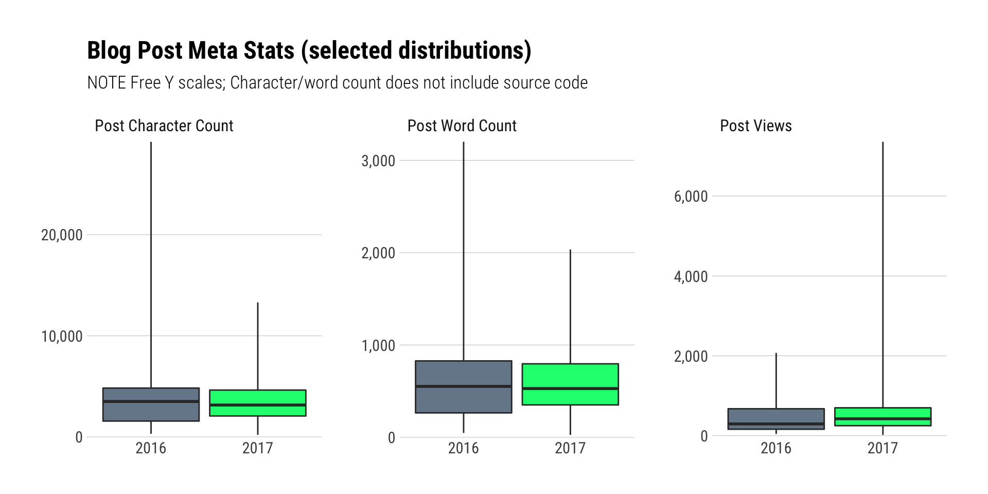
While I wanted to see my top posts each month, I decided to have some fun with this visualization. It packs-in the views for every JetPack-tracked posted written since January 1, 2016. I highlighted posts written in each month in 2017 in spring green. Astute readers (if you’ve made it this far) will note the use of Helvetica vs Roboto Condensed for the title & views annotations. Helvetica was the only tolerable (free) choice I had that included superscript 6. Check the code block for how I managed to get the in-month green dots on top.
I owe @henrikbengtsson an adult beverage or three for his assistance in ensuring this chart wasn’t too confusing. His annotation help was/is most appreciated.
mutate(wp_two_years, months = map(post_stats, ~{
  mos <- .x$years[[1]][[as.character(params$curr_year)]]$months
  data_frame(
    month = as.Date(sprintf("%s-%02d-01", params$curr_year,
                            as.integer(names(mos)))),
    count = as.integer(unname(.x$years[[1]][[as.character(params$curr_year)]]$months))
  )
})) %>%
  select(post_id, months) %>%
  unnest() %>%
  filter(count > 0) -> by_month

group_by(by_month, month) %>%
  top_n(1, count) %>%
  ungroup() %>%
  arrange(month) %>%
  left_join(wp_two_years, by="post_id") -> top_post_by_month

# this sure made the ggplot2 call less cumbersome
wrap_it <- function(title, count) {
  map2_chr(title, count,
           ~sprintf("%s\n[Views: %s]",
                    paste0(stri_wrap(urltools::url_decode(.x), 12), collapse="\n"),
                    scales::comma(.y))
  )
}

group_by(wp_two_years, date) %>%
  arrange(date) %>%
  mutate(month = as.Date(format(date, "%Y-%m-01"))) %>%
  ungroup() %>%
  select(post_id, originated_in_month=month) -> origin

left_join(by_month, origin, by="post_id") %>%
  mutate(written_in_month = (originated_in_month == month)) -> by_month
ggplot() +
geom_quasirandom(data=by_month,
aes(month, count, fill=written_in_month),
color="#2b2b2b", size=2.25, shape=21) +
geom_label(data=top_post_by_month,
aes(x=month, y=count, label=wrap_it(title, count)),
size=2.75, family="Helvetica", vjust=0, nudge_y=0.2,
lineheight=0.9, label.size=0) +
scale_x_date(date_breaks="1 month",
date_labels="%b\n%Y") +
scale_y_comma(expand=c(0,0.5),
trans="log10",
breaks=c(1, 10, 100, 1000, 10000, 100000),
limits=c(1, 100000)) +
scale_fill_manual(name=NULL,
values=c(`TRUE`="springgreen", `FALSE`="lightslategray"),
labels=c(sprintf("Not written in-month shown"),
sprintf("Written in-month shown"))) +
labs(
x=NULL, y="# In-month Views (according to JetPack)",
title=sprintf("Monthly Post View Count Distribution By Month (for posts created %s-%s)",
params$curr_year-1, params$curr_year),
subtitle="One dot == one post; Annotated by top post created in-month & written-in 2017 with [Views:]",
caption="NOTE: Y-axis log10 scale"
) +
theme_ipsum_rc(grid="Y") +
theme(legend.direction="horizontal") +
theme(legend.text.align=1) +
theme(legend.justification="right") +
theme(legend.position=c(1, 1)) -> gg
# to get the green dots on top we build the plot
# find the gree dots
# extract the calculated data for them
# trans back the data
# add a minimal point geom
gb <- ggplot_build(gg)
tbl_df(gb$data[[1]]) %>%
filter(fill=="springgreen") %>%
mutate(x=as.Date(x, origin="1970-01-01"), y=10^y) -> pt_dat
gg + geom_point(data=pt_dat, aes(x=x, y=y, fill="TRUE"), shape=21, size=3)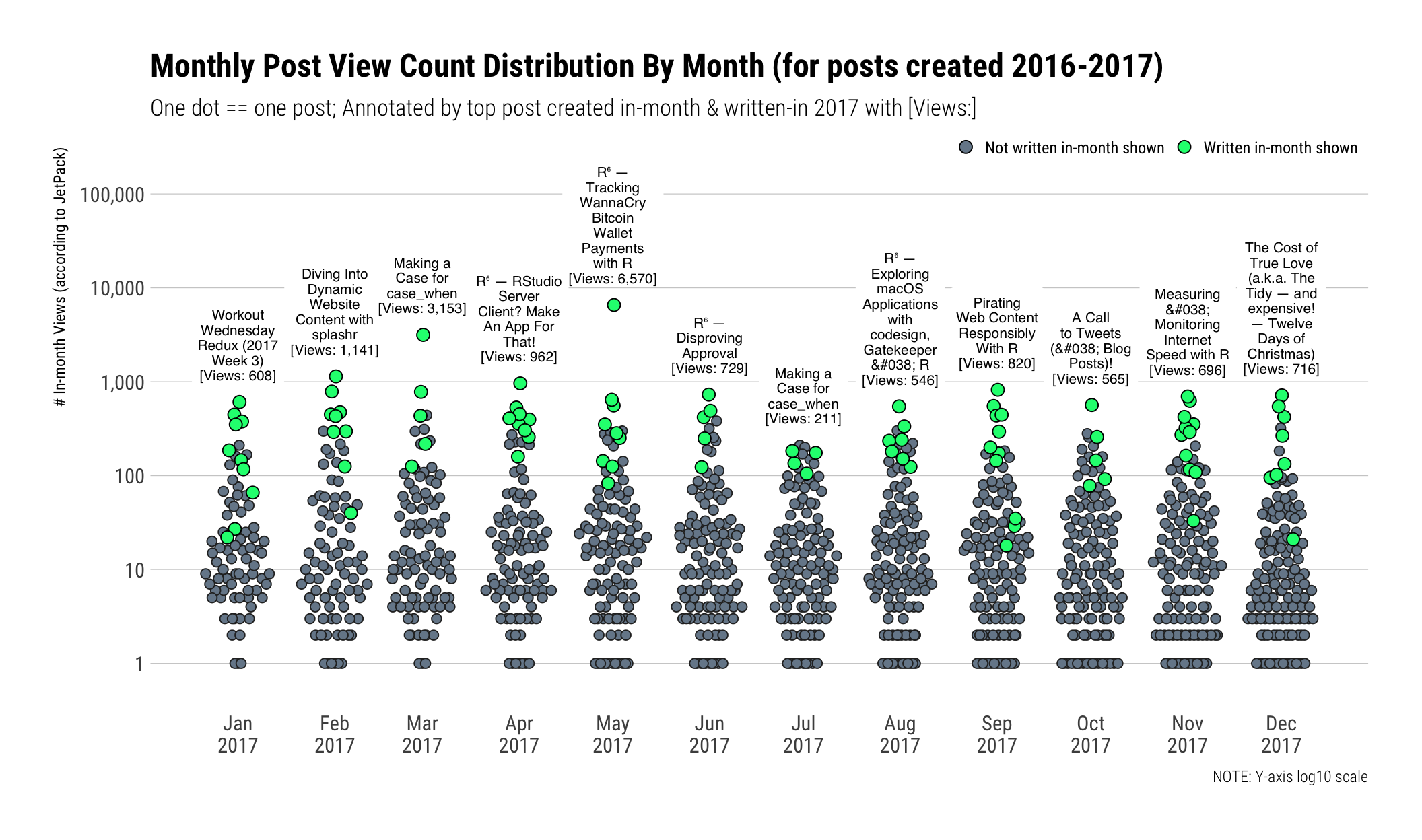
Reflection & Speculation
I blogged more but fell victim to my long-form post style (again). I really want to do more short posts in 2018 and will likely not blog much in the first half of the year, but hope to augment book-ish things with some useful blogs. I will very likely dual-purpose the existing blog for the book vs start a book-centric blog and may need to augment this Rmd next year to account for the fact that book-ish things will be intertwined with GH and WP (and, even Twitter) activity.
twitter_data_file <- file.path(rt, "data", "tweets.rds")
if (!file.exists(twitter_data_file)) {
  tweets <- read_csv(file.path(rt, "data", "tweets.csv")) # download your archive and rename it to this.
  write_rds(tweets, twitter_data_file)
} else {
  tweets <- read_rds(twitter_data_file)
}

mutate(tweets, day = as.Date(timestamp)) %>%
  mutate(year = lubridate::year(day)) %>%
  mutate(month = as.Date(format(day, "%Y-%m-01"))) -> tweets

filter(tweets, year %in%
         c(params$curr_year-1, params$curr_year)) -> tweets_two_years
I could have gone crazy here but virtually any of us on Twitter can go to Twitter’s analytics page and see Tweet data. And, while I would have liked to use rtweet, the “download my complete twitter archive” was just too easy to pass up. You can do that as well and just plug-in the data file to replicate this (fingers-crossed).
This one was somewhat interesting since it clearly showed the impact Murica arguing about and electing a baffoon had on me:
count(tweets_two_years, month) %>%
  ggplot(aes(month, n)) +
  stat_xspline(geom="area", color="slateblue", fill="slateblue",
               size=1, alpha=2/3) +
  scale_x_date(expand=c(0,0),
               date_breaks = "3 months",
               date_labels = "%b\n%Y") +
  scale_y_comma(expand=c(0,0), limits=c(0, NA)) +
  labs(x=NULL, y="# Tweets", title="Tweets per Month",
       subtitle="I took the election cycle pretty hard, but this truly made me realize just how hard.") +
  theme_ipsum_rc(grid="XY") +
  theme(axis.text.x=element_text(hjust=c(0, rep(0.5, 6), 1))) +
  theme(axis.text.y=element_text(vjust=c(0, rep(0.5, 2), 1)))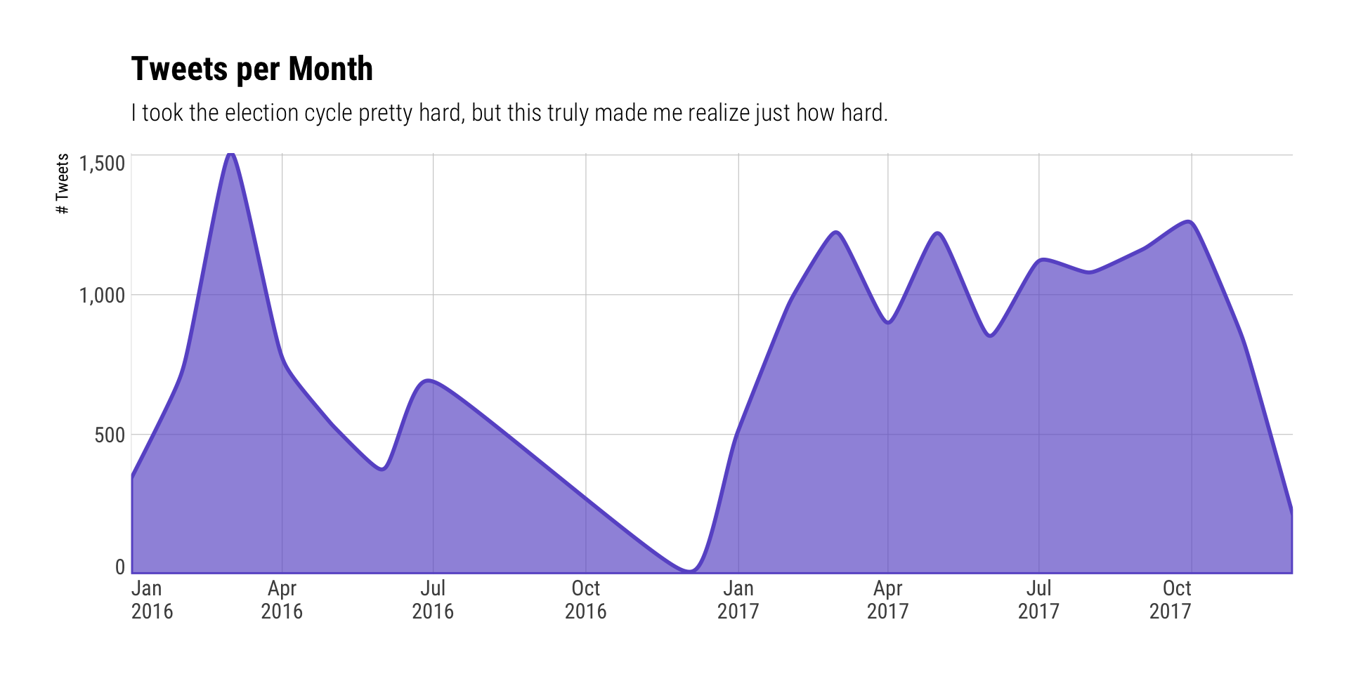
I’ve been obesessing a bit on Tweet length distribtions since Twitter increased the limit. I knew I pushed the 280 limit a bit this quarter and wanted to see by just how much. However, my first reaction to this char was: “Wow. I really went dark.”
I fear that I’ll over-blather to 280 more than I should when Twitter decides to grace us macOS folks with a desktop app that can support 280 characters.
mutate(tweets_two_years, `Tweet Length`=nchar(text)) %>%
  mutate(year = factor(year)) %>%
  ggplot(aes(month, `Tweet Length`)) +
  geom_hline(yintercept=140, linetype="dotted", size=0.25, color="#2b2b2b") + # this far and no further
  geom_quasirandom(aes(fill=year), size=1, shape=21, color="white", stroke=0.1) +
  scale_x_date(expand=c(0,0), date_breaks="1 month", date_labels="%b\n%Y") +
  scale_y_comma(breaks=c(seq(0, 280, 70)), limits=c(0, 320)) +
  scale_fill_manual(name=NULL, values=c("lightslategray", "springgreen"), guide=FALSE) +
  labs(x=NULL, title="Tweet Length Distribution (2 years)",
       subtitle="NOTE: Length can go over max limit due to how Twitter's API includes URLs\nI will likely refer to these as Twitter 'Dagger Charts' in 2018") +
  theme_ipsum_rc(grid="Y", axis_text_size=8)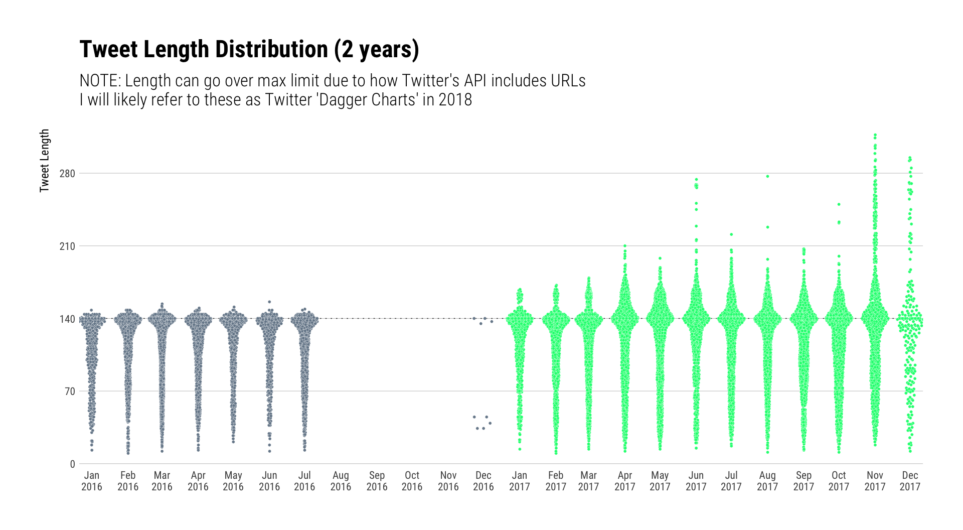
filter(tweets_two_years, !is.na(expanded_urls)) %>%
  select(year, expanded_urls) %>%
  mutate(year = factor(year)) %>%
  separate_rows(expanded_urls, sep=",h") %>%
  mutate(expanded_urls = stri_replace_first_regex(expanded_urls, "^ttp", "http")) %>%
  mutate(domain = domain(expanded_urls)) %>%
  mutate(domain = ifelse(domain == "l.dds.ec", "bit.ly", domain)) %>%  # spam domain takover == can't legitimately show this domain
  count(year, domain, sort=TRUE) -> tw_doms

count(tw_doms, year, wt=n) %>%
  mutate(lab=sprintf("%s\n(# URLs shared: %s)", year, scales::comma(nn))) %>%
  pull(lab) -> dom_year_sum
I seem to have re-tweeted or twitter-linked way more this year than last year (yes, I brought this somewhat ineffective chart-type back for a brief reprise). GitHub-ish domains are up there for both years and I can squint and see the New York Times trying to get above the fray, too. But, there are quite a number of domains in the “word soup” at the bottom and just focusing on the domain.tld doesn’t really help much (I tried).
ggplot(tw_doms) +
  geom_text(aes(year, n, label=domain, size=n, color=year), position="jitter") +
  scale_x_discrete(labels=dom_year_sum) +
  scale_y_sqrt(label=scales::comma) +
  scale_color_manual(name=NULL, values=c("lightslategray", "slateblue"), guide=FALSE) +
  scale_size(range=c(1.5, 6), guide=FALSE) +
  labs(x=NULL, y="# URLs shared", title="Domains of URLs Shared (2 years)", subtitle="NOTE: Y-axis sqrt") +
  theme_ipsum_rc(grid="XY")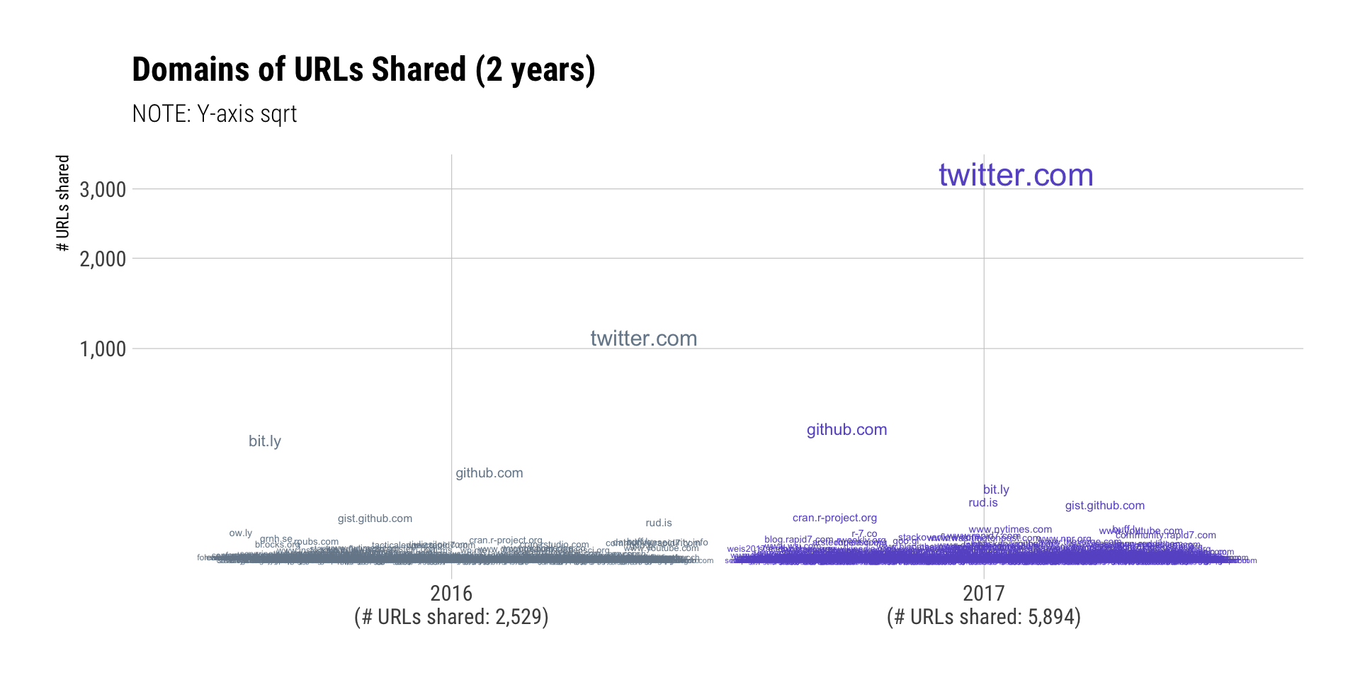
Reflection & Speculation
I’m not optimistic that Twitter will get better in 2018. One thing I can do to help it is to not tweet about politics. It clearly doesn’t do any good and a thoughtful long-form post would be a better use of time if the topic warrants exposition. The Library of Congress will also stop archiving all tweets next year, so history will be better served getting content into the global caches of The Internet Archive and Google.
I try to promote the work of others now and will redouble those efforts in 2018. But, there’s a down-side to that which this light analysis showed me: I visit far too many sites. I try to make a conscious decision to only hit up a few sites since the internet is truly fraught with peril. I’ve got a regularly updated hosts file that would make advertising executives across the world want to commit Hari Kari if everyone adopted it. I run uBlock origin and add custom rules to it regularly. I use a security-centric DNS configuration and I have more than a few endpoint protections active. Even with those precautions, there’s no way I was fully protected when I hit those ~1,100 domains and I shared links to folks who do not have the same set of precautions in place.
I’m not sure what I’m going to do about this, but it’s made me realize I’m not as picky as I thought I was and I definitely need a better workflow to help ensure the safety of folks I redirect.
FIN
That wraps up this data-driven year-in-review. It’s far from perfect, but I dug into some things I wanted to know and hopefully provided enough code and expository to help others do the same (or better!).
Let’s hope and pray 2018 has far better things in store for us all than the past two years have sent our collective way.
A blessed & contented New Year to you all!
# All the packages that ended up being used directly or by loading other packages
#
#  anytime      * 0.3.0      2017-06-05
#  ash            1.0-15     2015-09-01
#  assertthat     0.2.0      2017-04-11
#  backports      1.1.1      2017-09-25
#  base         * 3.4.3      2017-12-06
#  beeswarm       0.2.3      2016-04-25
#  bindr          0.1        2016-11-13
#  bindrcpp     * 0.2        2017-06-17
#  broom          0.4.3      2017-11-20
#  cellranger     1.1.0      2016-07-27
#  cli            1.0.0      2017-11-05
#  colorspace     1.3-2      2016-12-14
#  compiler       3.4.3      2017-12-06
#  crayon         1.3.4      2017-09-16
#  curl           3.0        2017-10-06
#  datasets     * 3.4.3      2017-12-06
#  devtools       1.13.4     2017-11-09
#  digest         0.6.13     2017-12-14
#  dplyr        * 0.7.4      2017-09-28
#  DT             0.2        2016-08-09
#  evaluate       0.10.1     2017-06-24
#  extrafont      0.17       2014-12-08
#  extrafontdb    1.0        2012-06-11
#  forcats      * 0.2.0      2017-01-23
#  foreign        0.8-69     2017-06-22
#  ggalt        * 0.5.0      2017-08-30
#  ggbeeswarm   * 0.6.0      2017-08-07
#  ggforce        0.1.1      2016-11-28
#  ggplot2      * 2.2.1.9000 2017-12-19
#  ggraph       * 1.0.0      2017-02-24
#  ggrepel        0.7.0      2017-09-29
#  gh           * 1.0.1      2017-09-01
#  glue           1.2.0.9000 2017-12-19
#  graphics     * 3.4.3      2017-12-06
#  grDevices    * 3.4.3      2017-12-06
#  grid           3.4.3      2017-12-06
#  gridExtra      2.3        2017-09-09
#  gtable         0.2.0      2016-02-26
#  haven          1.1.0      2017-07-09
#  hms            0.4.0      2017-11-23
#  hrbrthemes   * 0.5.0      2017-12-21
#  htmltools      0.3.6      2017-04-28
#  htmlwidgets    0.9        2017-07-10
#  httr           1.3.1      2017-11-14
#  igraph       * 1.1.2      2017-07-21
#  jericho      * 0.2.0      2017-09-05
#  jerichojars  * 3.4.0      2017-09-05
#  jsonlite       1.5        2017-06-01
#  KernSmooth     2.23-15    2015-06-29
#  knitr          1.17.20    2017-12-04
#  labeling       0.3        2014-08-23
#  lattice        0.20-35    2017-03-25
#  lazyeval       0.2.1      2017-10-29
#  lubridate    * 1.7.1      2017-11-03
#  magrittr       1.5        2014-11-22
#  maps           3.2.0      2017-06-08
#  MASS           7.3-47     2017-02-26
#  memoise        1.1.0      2017-04-21
#  methods      * 3.4.3      2017-12-06
#  mnormt         1.5-5      2016-10-15
#  modelr         0.1.1      2017-07-24
#  munsell        0.4.3      2016-02-13
#  nlme           3.1-131    2017-02-06
#  openssl        0.9.9      2017-11-10
#  parallel       3.4.3      2017-12-06
#  pkgconfig      2.0.1      2017-03-21
#  plyr           1.8.4      2016-06-08
#  pressur      * 0.1.0      2017-12-27
#  proj4          1.0-8      2012-08-05
#  psych          1.7.8      2017-09-09
#  purrr        * 0.2.4      2017-10-18
#  R6             2.2.2      2017-06-17
#  RApiDatetime   0.0.3      2017-04-02
#  RColorBrewer   1.1-2      2014-12-07
#  Rcpp           0.12.14    2017-11-23
#  readr        * 1.1.1      2017-05-16
#  readxl         1.0.0      2017-04-18
#  reshape2       1.4.3      2017-12-11
#  rJava        * 0.9-9      2017-10-12
#  rlang          0.1.4.9000 2017-12-19
#  rmarkdown      1.8        2017-11-17
#  rprojroot    * 1.2        2017-01-16
#  rstudioapi     0.7        2017-09-07
#  Rttf2pt1       1.3.4      2016-05-19
#  rvest          0.3.2      2016-06-17
#  scales         0.5.0.9000 2017-11-20
#  stackr       * 0.0.0.9000 2017-12-21
#  stats        * 3.4.3      2017-12-06
#  stringi      * 1.1.6      2017-11-17
#  stringr      * 1.2.0      2017-02-18
#  tibble       * 1.3.4      2017-08-22
#  tidyr        * 0.7.2      2017-10-16
#  tidyselect     0.2.3      2017-11-06
#  tidyverse    * 1.2.1      2017-11-14
#  tools          3.4.3      2017-12-06
#  triebeard      0.3.0      2016-08-04
#  tweenr         0.1.5      2016-10-10
#  udunits2       0.13       2016-11-17
#  units          0.4-6      2017-08-27
#  urltools     * 1.6.0      2016-10-17
#  utils        * 3.4.3      2017-12-06
#  vipor          0.4.5      2017-03-22
#  viridis        0.4.0      2017-03-27
#  viridisLite    0.2.0      2017-03-24
#  waffle         0.8.0      2017-09-24
#  withr          2.1.0.9000 2017-12-19
#  xml2           1.1.9000   2017-12-01
#  yaml           2.1.15     2017-12-01